Nusselt number to describe convective heat transfer

The Nusselt number is a dimensionless similarity parameter to describe convective heat transfer, independent of the size of the system.

Introduction

Convective heat transfer describes the heat transport between a solid surface and a flowing fluid. The greater the temperature difference between the solid wall and the flowing fluid, the greater the heat flow transferred. The relationship between temperature difference and heat flux is quantified by a so-called heat transfer coefficient α:

\begin{align}
\label{qq}
&\boxed{\dot q_\alpha = \alpha \cdot (T_w-\overline{T_f})} ~~~~~\text{convective heat transfer} \\[5px]
\end{align}

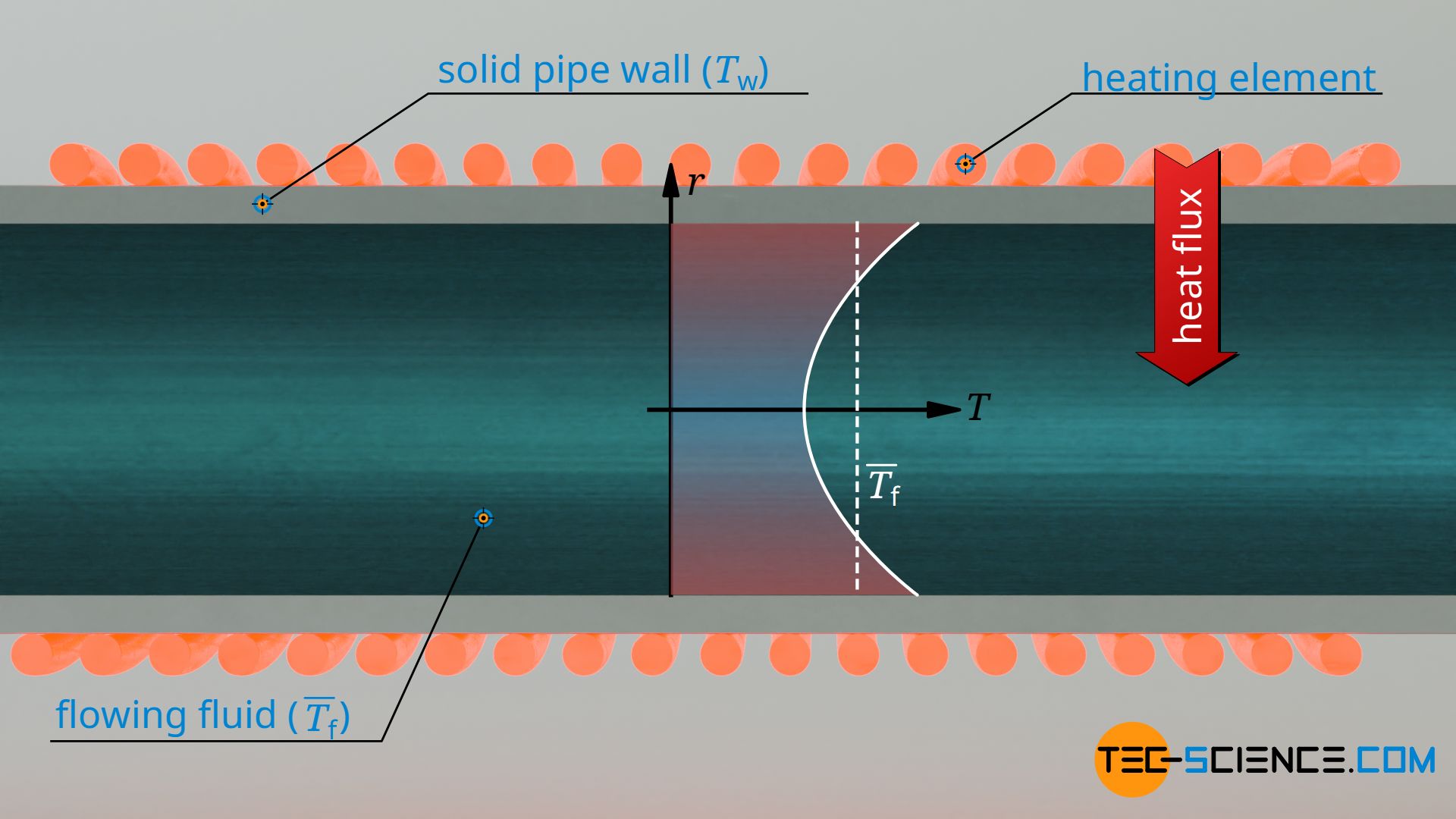
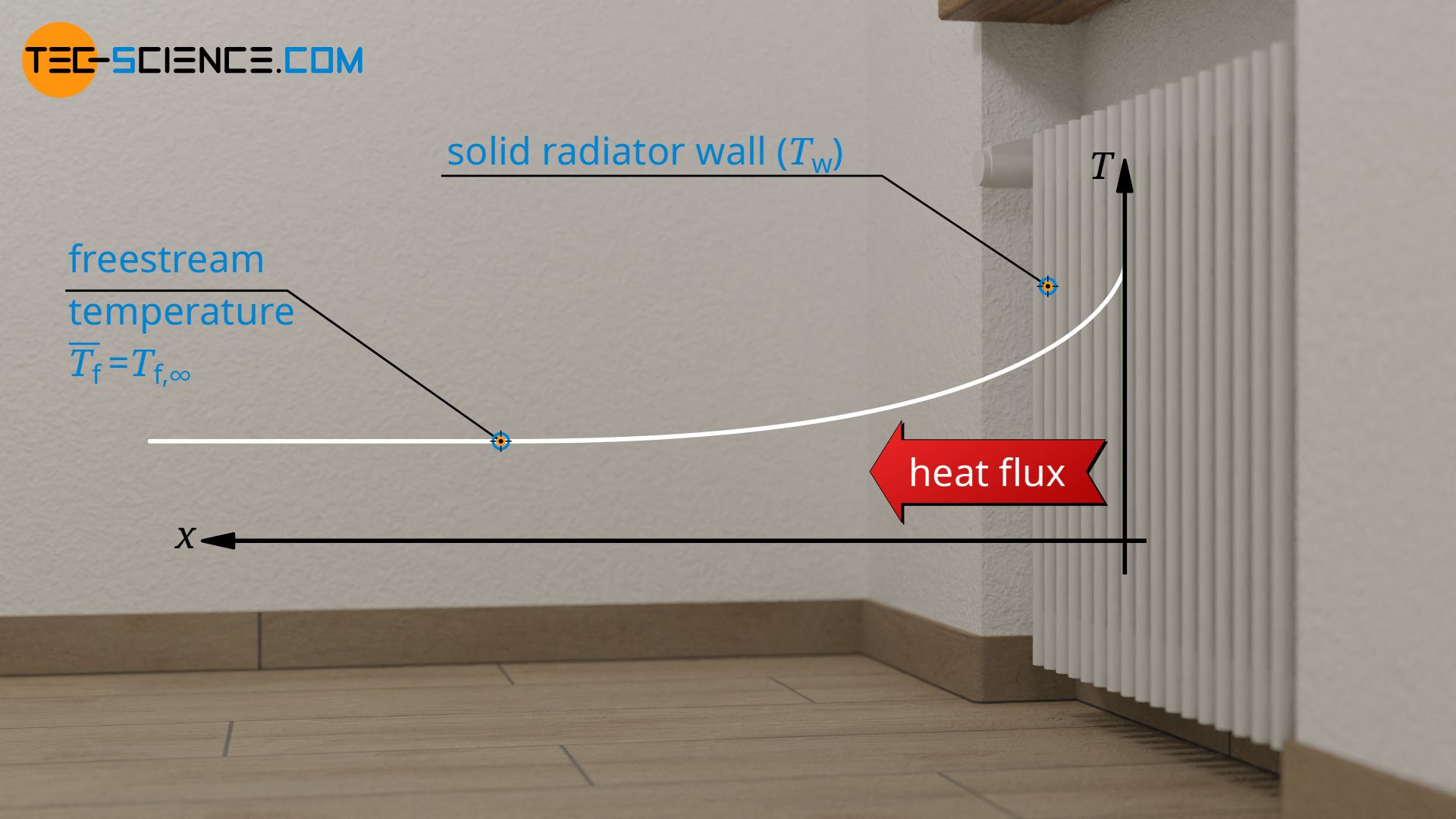
In this formula, q* denotes the heat flux at the wall, T_f is the temperature of the flowing fluid and T_w the temperature of the wall. For a pipe flow, fluid temperature refers to the adiabatic mixing temperature, i.e. to the temperature when the fluid would be ideally mixed at the point of interest. In an free flow (for example the flow of air past a radiator), the fluid temperature refers to the temperature in the freestream, i.e. at a sufficiently large distance from the wall (T_f=T_f,∞).

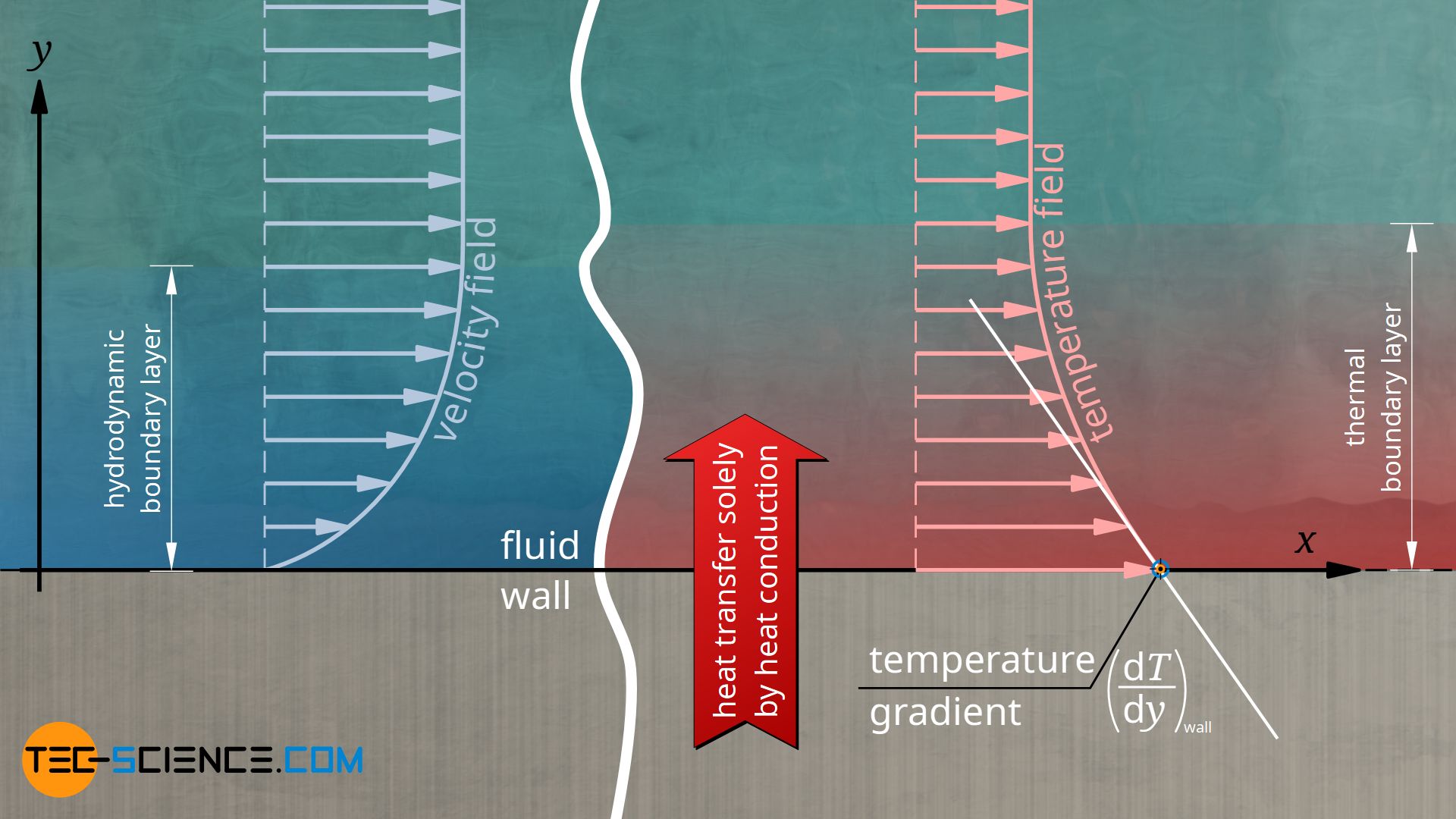
In the article on the heat transfer coefficient, the importance of the boundary layer between flowing fluid and solid wall has already been explained in detail. For this reason, it will be dealt with here only briefly. Due to the so-called no-slip condition, the fluid adheres directly to the wall (this applies only to fully developed flows!). Thus, heat transport between wall and fluid at this point is only possible by thermal conduction. According to Fourier’s law, the temperature gradient in the fluid has a decisive influence on the heat flow. The greater the temperature gradient, the higher the heat flow or heat flux:

\begin{align}
\label{qw}
& \boxed{\dot{q_\lambda} =- \lambda_f \cdot \left(\frac{\text{d}T_f}{\text{d}y}\right)_\text{wall}} ~~~~~\text{Fourier’s law} \\[5px]
\end{align}

The thermal conductivity of the fluid is denoted by λ_f and the term dT_F/dy|_wall represents the temperature gradient of the fluid directly at the wall. With the condition q_λ*=q_α*, the below given relationship results for the heat transfer coefficient α. Note that the heat fluxes at the wall must be identical, because only as much heat can be passed through the fluid as the wall gives off.

\begin{align}
&\alpha = \frac{\dot q_\alpha}{T_w-\overline{T_f}} \\[5px]
\label{wand}
&\boxed{\alpha = \frac{- \lambda_f \cdot \left(\frac{\text{d}T_f}{\text{d}y}\right)_\text{wall}}{T_w-\overline{T_f}}}\\[5px]
\end{align}

Compared to a fluid at rest (no convection), a flow now has a decisive influence on the temperature field in the fluid, which in turn has an effect on the temperature gradient and thus on the overall (convective) heat transfer. Under simplified conditions we consider a heated wall, which transfers heat to a passing fluid at a point x. Due to the flow of the fluid, the heat transferred to the fluid is transported away relatively quickly and cooler fluid flows in. If, on the other hand, the fluid would not flow, the heat would accumulate, so to speak, and the fluid would heat up relatively strongly.

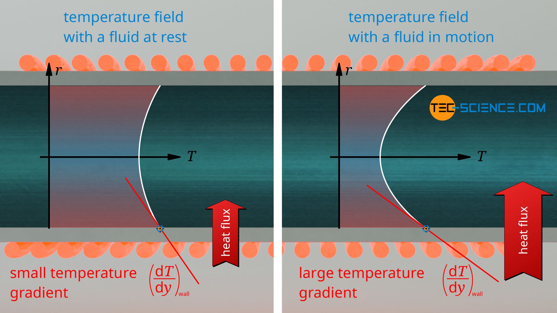
In other words, a flowing fluid near a heated wall is cooler than a fluid at rest. Thus, with convection, the temperature in the fluid drops more strongly directly at the wall. This in turn means a greater heat flow according to Fourier’s law. Particularly large temperature gradients are obtained when the flow is turbulent, so that the fluid mixes and heat is transported away from the wall much faster.

Definition of the Nusselt number

As just explained, the heat transport directly at the wall takes place exclusively through thermal conduction. Heat conduction however takes place not only at the wall, but within the whole fluid. The mechanism of heat conduction is not eliminated just because the fluid moves. However, at greater distances from the wall, heat transport by convection dominates. However, as the above mentioned example with the heated wall showed, both mechanisms of heat transfer influence each, because the temperature field is changed by the flow.

In summary, it can be said that convection is essentially based on two mechanisms of heat transfer:

• thermal conduction through random molecular motion of molecules (dominant near the wall, where the fluid rests)
• thermal convection through ordered molecular motion of the molecules – bulk motion (dominant at larger distances from wall)
• (thermal radiation only plays a role at extremely high temperature differences and is therefore neglected)

Both mechanisms together define the observable heat transfer by convection, which is described macroscopically by equation (\ref{qq}) and can also be expressed microscopically by equation (\ref{qw}).

The ratio between real present convective heat transfer (“α”) and a pure fictitious heat conduction (“λ_f“), is given by the dimensionless Nusselt number “Nu”:

\begin{align}
\label{nu}
&\boxed{Nu:= \frac{\alpha}{\lambda_f}L} ~~~~~\text{Nusselt number} \\[5px]
\end{align}

In this formula, L denotes the so-called characteristic length of the system, which describes the influence of the system size on the heat transfer. In the case of a pipe, the characteristic length would correspond to the pipe diameter. When considering the convective heat transfer at a plate, the characteristic length equals the length of the plate in the direction of flow.

The Nusselt number describes the ratio of convective heat transfer compared to pure heat conduction!

At this point it is often tried to give a clear interpretation of the Nusselt number as the ratio of convection to conduction. In special cases this may indeed be possible. In most cases, however, this leads to more confusion than it contributes to a clear understanding (in our opinion). Therefore we would like to take a different approach. For this purpose we take the heat transfer coefficient according to equation (\ref{wand}) and put it into the definition of the Nusselt number (\ref{nu}):

\begin{align}
\require{cancel}
&Nu= \frac{\alpha}{\lambda_f}L \\[5px]
&Nu= \underbrace{\frac{- \cancel{\lambda_f} \cdot \left(\frac{\text{d}T_f}{\text{d}y}\right)_\text{wall}}{T_w-\overline{T_f}}}_{\alpha} \cdot \frac{L}{\cancel{\lambda_f}} \\[5px]
\label{nutint}
&\boxed{Nu= \color{red}{\frac{\left(\frac{\text{d}T_f}{\text{d}y}\right)_\text{wall}}{\overline{T_f}-T_w}} \cdot L} \\[5px]
\end{align}

The term marked in red corresponds to a normalized temperature gradient at the wall. The Nusselt number can therefore be interpreted as a measure of a dimensionless temperature gradient on the wall. And the greater this temperature gradient, the higher the heat flow. Later we will show that for fully developed pipe flows this dimensionless temperature gradient is constant under certain boundary conditions. This then also applies to the Nusselt numbers.

The Nusselt number is a measure of the (dimensionless) temperature gradient of the fluid at the wall!

Importance of the Nusselt number in practice

As strange as it may sound at first, the Nusselt number gets its true meaning only from the concept of similitude. Because only if the same Nusselt numbers are obtained in systems of different sizes can similar heat transfers by convection be assumed. It is therefore possible to first determine the Nusselt number in small model experiments and then apply the obtained Nusselt number to the real system with its characteristic length:

\begin{align}
\label{alpha}
&\boxed{\alpha = Nu \cdot \frac{\lambda_f}{L}} \\[5px]
\end{align}

The Nusselt number is a dimensionless similarity parameter to describe convective heat transfer. Only with identical Nusselt Numbers one obtains physically similar heat transfers regardless of the system size.

Note: While the heat transfer coefficient α always refers to a concrete application (depending on the size of the system), the Nusselt number “Nu” describes convective heat transfer in general, regardless of the actual application and the size of the system.

The Nusselt number is therefore of great importance in chemical engineering, for example. Before chemical processes are carried out or plants are built on a real scale, they are first tested or researched on a smaller scale (e.g. in the laboratory or pilot plant). In order to obtain the same or similar heat transfer as later on in real life, the Nusselt number must be the same on all scales. So you determine the Nusselt number on a small scale and then apply it to the real scale (called scale-up).

In case of convective heat transfer, the Nusselt number is the link between model and real system!

Local and average Nusselt number

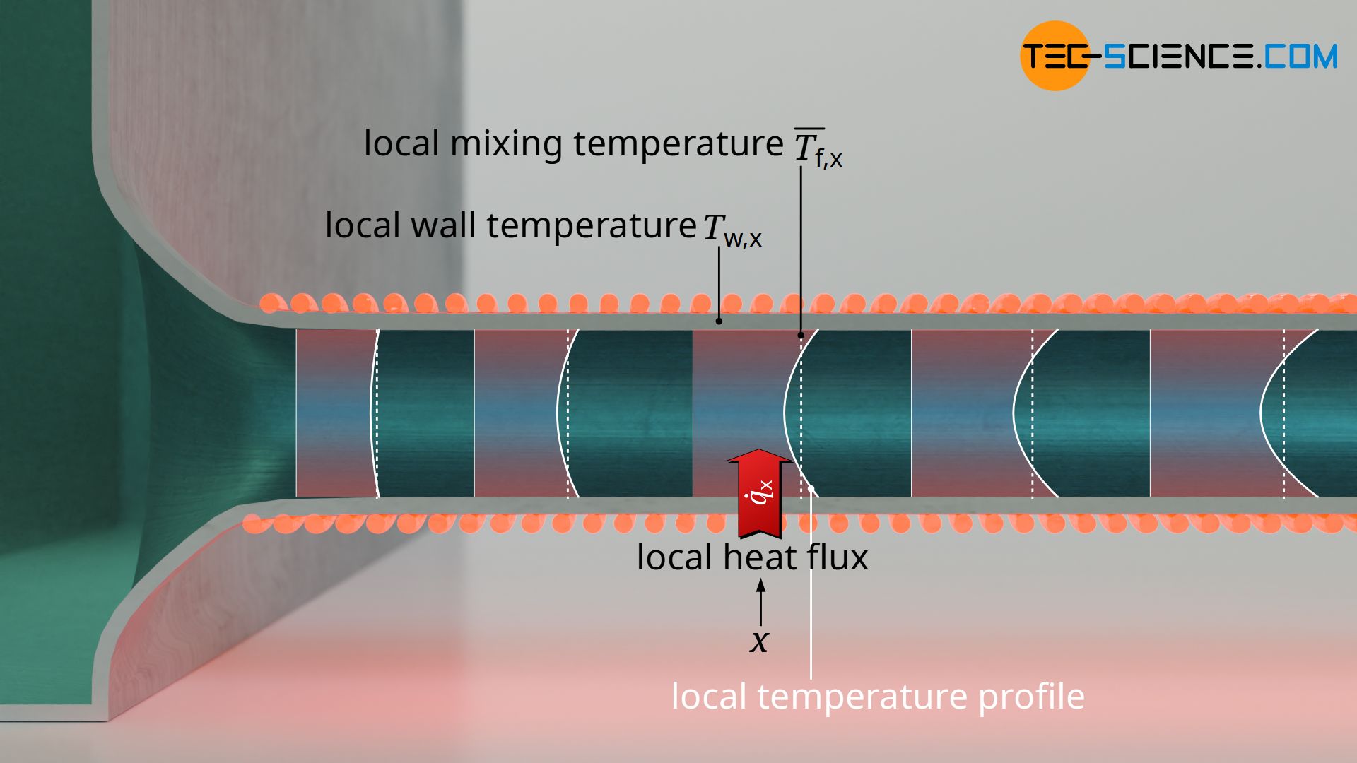
If one wants to describe the heat transfer only at a certain point x in a system (e.g. at a certain point in a pipe), then one also speaks of the local Nusselt number. The local Nusselt number thus describes the local heat transfer coefficient and thus the local heat flux.

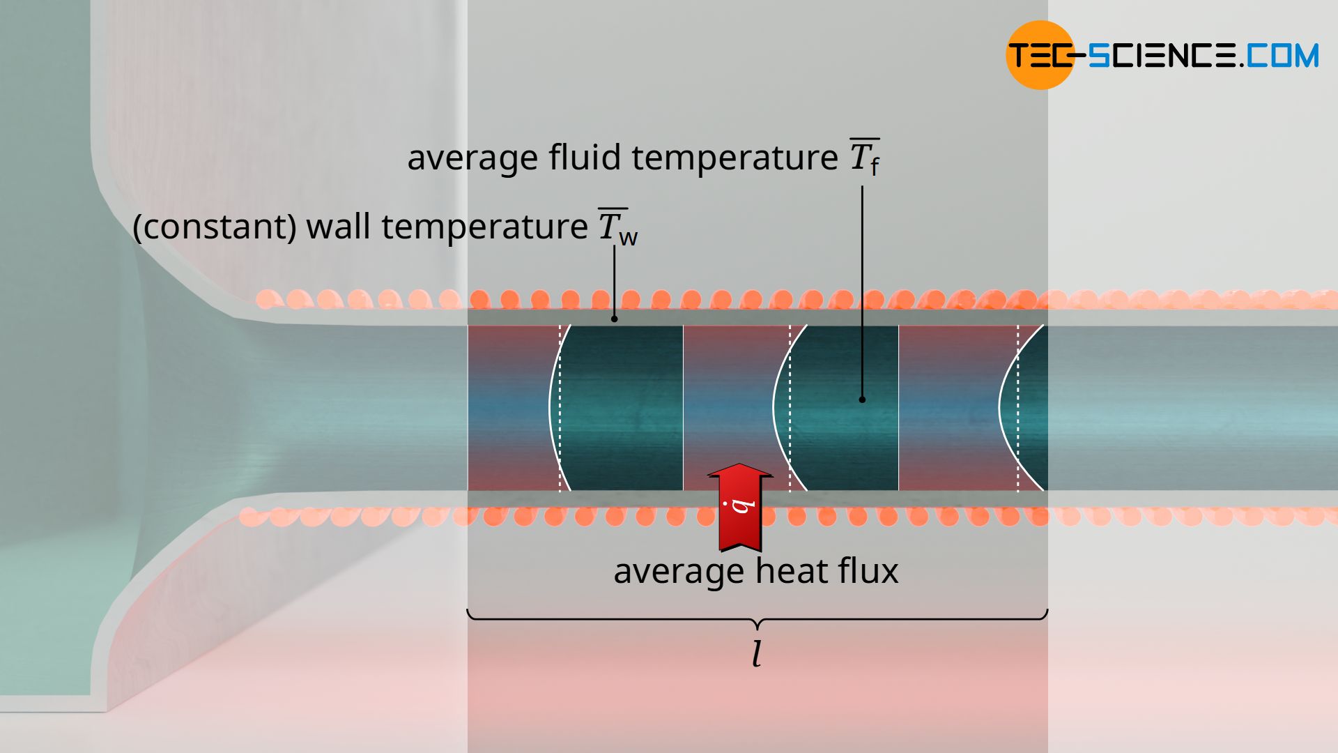
However, the heat transfer can also be related to the entire system as such or to a longer section. In the case of a pipe flow, this means that the Nusselt number no longer refers to a certain point in the pipe, but to the entire pipe itself or to a longer section of length l. In this context, one speaks of the average Nusselt number, which indicates the average heat transfer coefficient. In this case, one obtains the average heat flux of the entire pipe. The average Nusselt numbers are thus obtained by integrating the local Nusselt numbers.

In the article Calculation of the Nusselt Numbers, the calculation of the local and average Nusselt Numbers of flows over plates and through pipes is discussed in more detail.

Dimensionless temperature and Nusselt number in the context of pipe flows

The basic “problem” in describing the temperature profile inside a pipe is that the profile changes along the pipe. After all, in an isothermally heated pipe, heat is permanently transferred to the fluid, which heats up as a result. This means that the temperature difference between a point in the fluid at a distance r from the pipe axis (T_f) and the wall (T_w) is a function of r and the position x:

\begin{align}
&f(x,r) = T_f-T_w \\[5px]
\end{align}

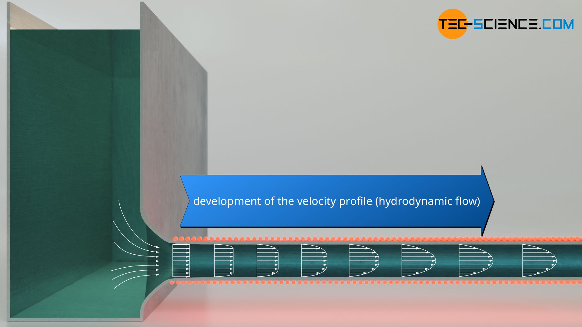
If, however, this function is related to the temperature difference between the mixing temperature at the considered location x (T_f) and the constant wall temperature T_w, then the obtained dimensionless fluid temperature θ_f is independent of the location in the pipe for a thermally and hydrodynamically fully developed flow. A flow is considered to be fully developed when the thickness of the boundary layers no longer changes.

\begin{align}
&\boxed{\theta_f:= \frac{T_f-T_w}{\overline{T_f}-T_w}} ~~~~~\text{dimensionless fluid temperature}\\[5px]
\end{align}

A fully developed flow is a flow in which the thickness of the boundary layers no longer changes!

Note that the wall temperature T_w is a constant in this equation, while the fluid temperature T_f is dependent on both r and x. The mixing temperature, however, is only a function of the location x:

\begin{align}
&\theta_f(r) = \frac{T_f(r,x)-T_w}{\overline{T_f}(x)-T_w} \\[5px]
\end{align}

Thus one has a dependence of x in the numerator of the fraction as well as in the denominator. Due to the quotient, the dependence of x is canceled out, so to speak, so that the entire term is ultimately no longer a function of x. However, due to the complexity, we do not want to prove that this is actually the case. However, we want to show that under this assumption that the Nusselt number is independent of x as well (and thus also the heat transfer coefficient).

For this purpose the dimensionless temperature gradient is determined by deriving the equation above with respect to r (partial derivative). Note that the term marked in blue is be considered a constant, since this term is not a function of r. Furthermore, the derivative of the wall temperature T_w with respect to r is zero, since the wall temperature is a constant.

\begin{align}
&\frac{\text{d} \theta_F(r)}{\text{d}r}= \color{blue}{\frac{1}{\overline{T_f}(x)-T_w}} \cdot \frac{\text{d}\left[T_f(r,x)-T_w\right]}{\text{d}r} \\[5px]
&\frac{\text{d} \theta_f(r)}{\text{d}r}= \color{blue}{\frac{1}{\overline{T_f}(x)-T_w}} \cdot \left[\frac{\text{d}T_f(r,x)}{\text{d}r} – \underbrace{\frac{\text{d}(T_w)}{\text{d}r}}_{=0} \right]\\[5px]
&\frac{\text{d} \theta_f(r)}{\text{d}r}= \color{blue}{\frac{1}{\overline{T_f}(x)-T_w}} \cdot \frac{\text{d}T_f(r,x)}{\text{d}r}\\[5px]
\end{align}

The following formula therefore applies to the dimensionless temperature gradient at the wall:

\begin{align}
&\left(\frac{\text{d} \theta_f(r)}{\text{d}r}\right)_\text{wall}= \frac{\left(\frac{\text{d}T_f(r,x)}{\text{d}r}\right)_\text{wall}}{\overline{T_f}(x)-T_w} \\[5px]
\end{align}

Let us omit the specification of the variables at this point,

\begin{align}
&\left(\frac{\text{d} \theta_f}{\text{d}r}\right)_\text{wall}= \color{red}{\frac{\left(\frac{\text{d}T_f}{\text{d}r}\right)_\text{wall}}{\overline{T_f}-T_w}} \neq f(x)\\[5px]
\end{align}

then it is immediately apparent that the expression on the right hand side of this equation corresponds to the term marked in red in equation (\ref{nutint}) (the variable y corresponds in this case to the radius r and the characteristic L to the inner diameter of the pipe d). However, as the left hand side of this equation shows, this term does not depend on x and therefore the Nusselt number is not a function of x:

\begin{align}
&\boxed{Nu= \left(\frac{\text{d} \theta_f}{\text{d}r}\right)_\text{wall} \cdot d} \neq Nu(x)\\[5px]
\end{align}

Note that the dimensionless temperature profile and the Nusselt number as well as the heat transfer coefficient are independent of the location x only under the following conditions:

• thermally and hydrodynamically fully developed laminar flow profile (see also Hagen-Poiseuille flow)
• constant wall temperature or constant heat flux at the wall

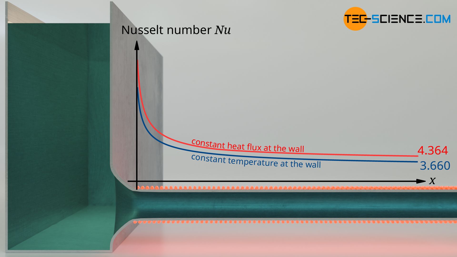
The longer a pipe is, the better the condition of fully developed pipe flow will be fulfilled. The Nusselt number therefore tends to approach a limit for long pipes. This asymptote can be determined by numerical methods. Depending on the boundary condition, the following asymptotes result for the local or average Nusselt numbers:

\begin{align}
\label{366}
&\boxed{Nu_{\infty}= 3,660} &&~~~\text{for constant wall temperature}\\[5px]
\label{4364}
&\boxed{Nu_{\infty}= 4,364} &&~~~\text{for constant heat flux at the wall}\\[5px]
\end{align}

Note that a fully developed flow profile theoretically exists only for very long pipes or at a sufficiently large distance from the beginning of the pipe. Therefore, the local Nusselt number generally depends on x and the average Nusselt number depends on the pipe length l. More about the calculation of those Nusselt numbers can be found in the article Calculation of the Nusselt Numbers.