The hydrodynamic boundary layer of a flow has a decisive influence on heat and mass transport.
Introduction
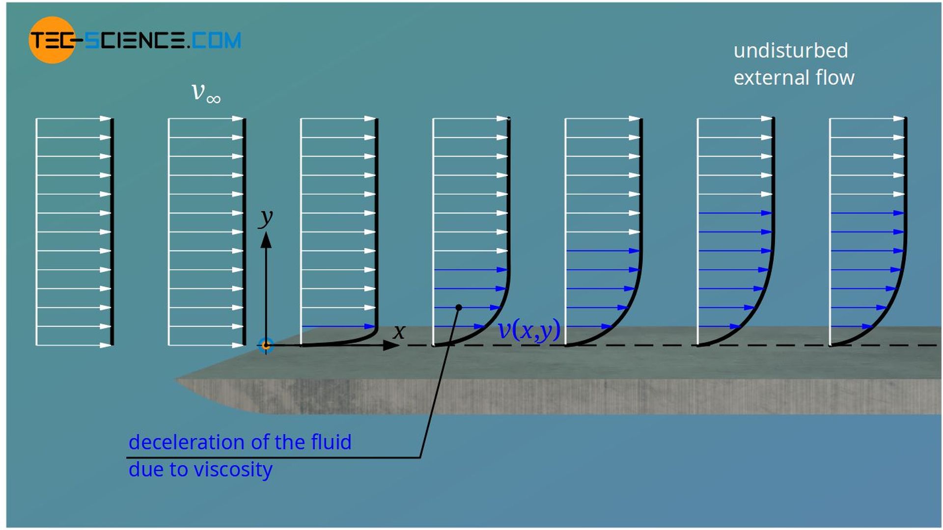
In this article we take a closer look at the boundary layers between a solid surface and a flowing fluid. Such boundary layers influence, for example, the convective heat transfer to a decisive extent. As an example we consider an isothermally heated plate with a temperature T0. A fluid flows over this plate. The constant velocity in the freestream is denoted by v∞. The temperature of the freestream is T∞.
Intermolecular forces within the fluid and frictional forces between fluid and solid surface influence the flow velocity. This results in the development of a typical velocity profile. Due to the frictional forces, the fluid molecules adhere to the wall, i.e. the speed of the flow is zero there (called no-slip condition). With increasing distance to the wall, the velocity increases. At a certain distance the flow velocity finally reaches the velocity v∞ of the freestream (“undisturbed flow”).
Influence of viscosity on the disturbance of the flow
How large that area is, up to where the flow reaches the undisturbed velocity (white arrows in the upper figure), depends mainly on the viscosity of the fluid. For fluids with low viscosity, such as water or gases, the intermolecular forces are relatively low. If you imagine the fluid to be made up of many small layers, the attraction between these layers is relatively low. This means that they do not hinder each other in their motion as much when they flow at different speeds. Fluids with low viscosity therefore reach the freestream velocity already at a relatively small distance from the wall.
Fluids with higher viscosities, such as oils, on the other hand, have relatively high intermolecular cohesion forces. The individual fluid layers therefore exert relatively strong forces of attraction on each other and strongly influence each other in their movement. This region within which the flow is disturbed is therefore larger for highly viscous fluids. This area where the flow velocity is disturbed by the influence of shear stresses between the fluid layers, is also called velocity boundary layer or hydrodynamic boundary layer.
The boundary area up to which the local flow velocity has reached 99 % of the velocity of the freeestream is also called velocity boundary layer or hydrodynamic boundary layer.
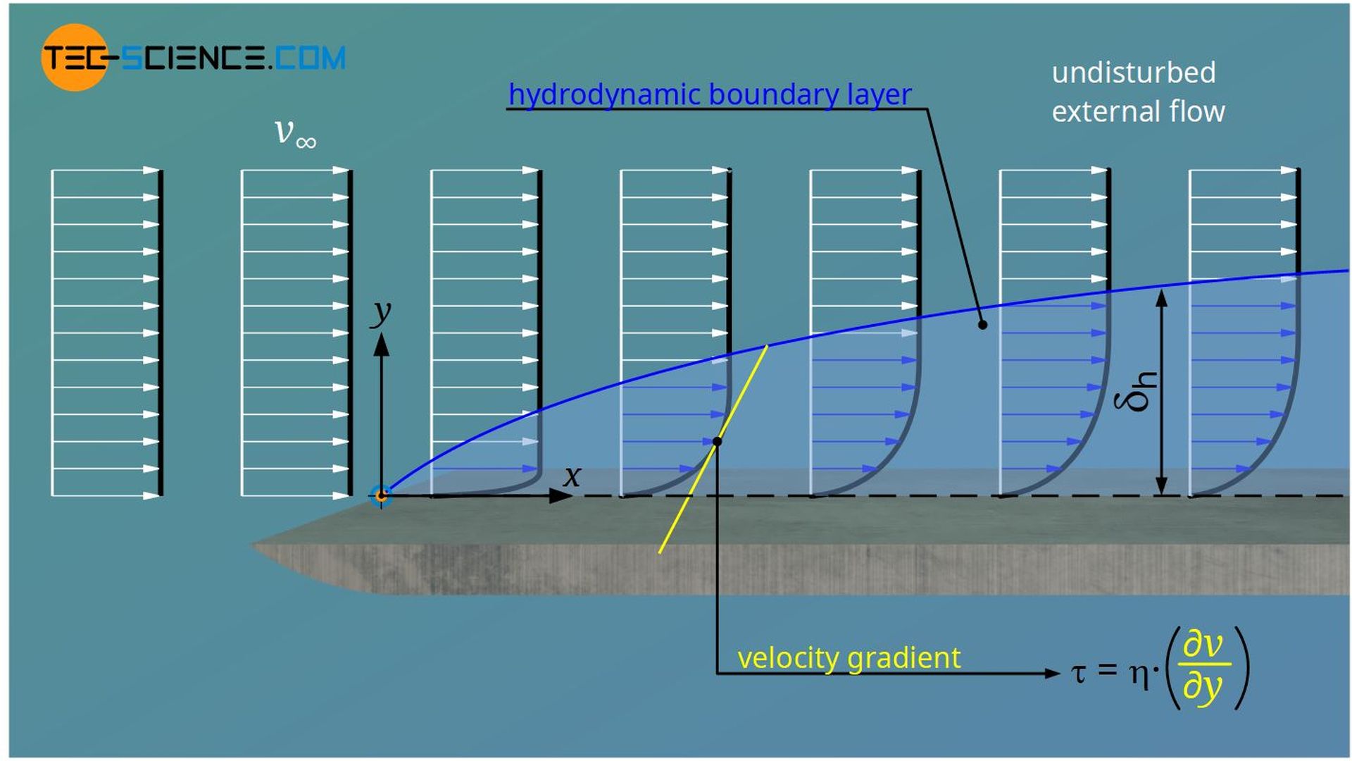
Velocity gradients and shear stresses
The hydrodynamic boundary layer is thus defined by the fact that within this layer velocity gradients and thus also shear stresses τ exist. Note that according to Newton’s law of fluid friction, the existence of velocity gradients always implies the existence of shear stresses:
“shear stress = viscosity x velocity gradient”
These shear stresses are ultimately responsible for the deceleration of the fluid layers and the subsequent formation of an equilibrium between the external pressure gradient (as a drive for the flow) and the shear stresses.
Since there are no velocity gradients outside the hydrodynamic boundary layer, the shear stresses are negligible. In this undisturbed flow, the viscosity of the fluid plays no role. But within the boundary layer, the shear stresses are usually no longer negligible and have a decisive influence on the flow. Even if the boundary layer is defined very precisely, the change of the properties of the flow inside and outside of this “sharp” boundary is smooth!
Course of the laminar boundary layer
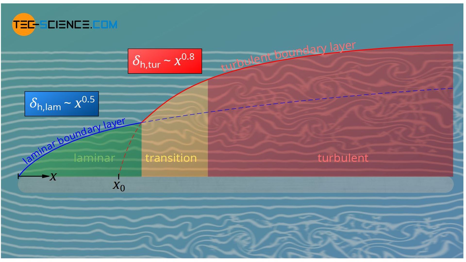
The thickness of the boundary layer increases with increasing distance from the leading edge of the plate, as more and more fluid layers come under the influence of friction. Each fluid layer gradually slows down the layer above it, so to speak. This is also known as startup flow. From a large enough distance, however, the thickness of the boundary layer δh then (almost) no longer changes. The aforementioned equilibrium between pressure gradient and frictional force has been reached. In this case one speaks of a completely developed boundary layer.
For a flow over a thin flat plate, the boundary layer equations can be solved analytically (Blasius solution). A further assumption is that the flow is laminar and incompressible and that there is no pressure gradient due to frictional forces along the plate. The thickness of the boundary layer δh at a distance x from the leading edge is then dependent on the local Reynolds number Rex and can be determined as follows:
\begin{align}
&\boxed{\delta_\text{h,lam}= \frac{5 \cdot x}{\sqrt{Re_x}}} ~~~Re_x = \frac{v_\infty \cdot x}{\nu}\\[5px]
&\boxed{\delta_\text{h,lam} \sim x^{0.5}} \\[5px]
\end{align}
In this formula, v∞ denotes the velocity of the freestream and ν (Greek small letter Nu) the kinematic viscosity of the fluid. In the case of water or air and a plate dimension in the order of 1 m and speeds in the range of several meters per second, the thicknesses of the boundary layers are thus in the order of 1 mm.
Transport of momentum
Shear stress influences the velocity of the flow (i.e. momentum of the flow), so that in connection with viscosity one also speaks of a transport of momentum or momentum diffusion. Such a transport of momentum takes place between the individual fluid layers, so that there is a corresponding change in the flow velocity in the individual fluid layers (see also the article Thermal and concentration boundary layer, in which an analogy to the other transport processes is shown).
And indeed, especially with gases, the viscosity is mainly due to such diffusion of fluid molecules into the neighboring fluid layers. Due to the random thermal motion, fluid particles from slow fluid layers, for example, diffuse into faster moving fluid layers. The slow fluid particles thus lead to a kind of deceleration of the faster fluid layers. The effect is ultimately the same as when frictional forces act in the form of cohesion forces between the layers. Such intermolecular forces are, however, only very weak in gases, so that the diffusion of fluid particles is the main cause of the viscosity of gases. The term momentum diffusion is indeed to be taken literally.
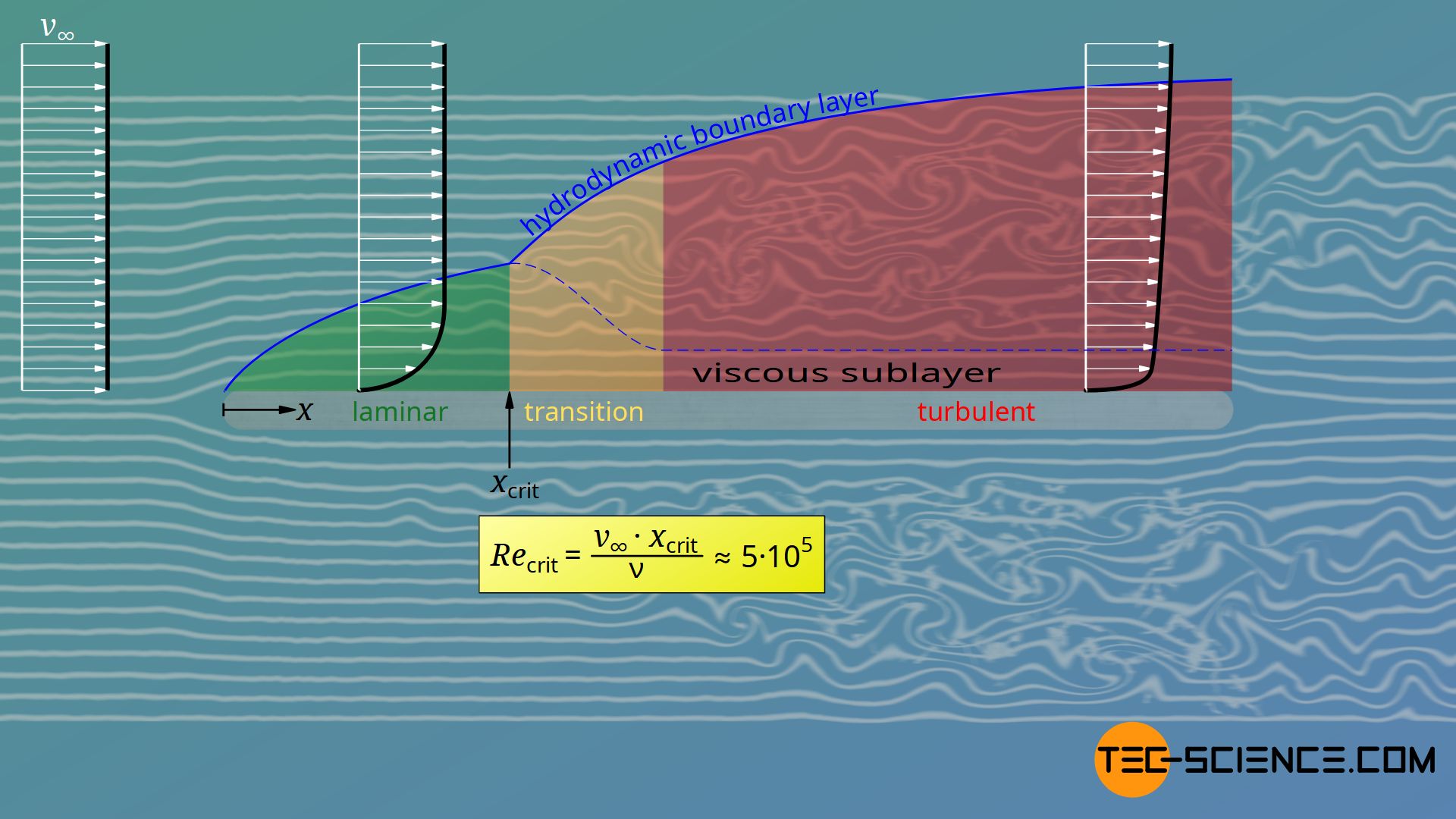
Laminar and turbulent boundary layer
Boundary layers can not only be laminar or turbulent, but also consist of a mixture of both types of flow. In fact, this usually occurs with bodies around which flow passes, as neither the body is optimally streamlined nor the surface is perfectly smooth. In addition, a flow is never perfectly laminar but always contains a certain degree of turbulence (i.e. small fluctuations of speed perpendicular to main flow direction). Even the Brownian thermal motion of the molecules already leads to a certain degree of turbulence, which thus serves as a disturbance.
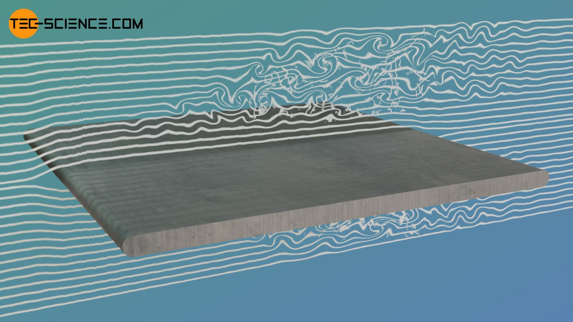
Let us now look again at our flat plate. So either there are already small disturbances in the flow or these are formed when the fluid flows onto the plate. Influenced by the boundary layer itself, the disturbances increasingly build up. To a certain degree, however, these disturbances can be compensated by the fluid. The higher the viscosity of the fluid (greater internal cohesion) and the lower the flow velocity (lower inertia forces), the easier it is for the fluid to compensate.
However, from a critical point xcrit the disturbances have increased to such an extent that they become unstable. The viscosity can no longer counteract the forces of inertia. The laminar flow changes to a turbulent flow after a relatively short transition range. This transition takes place at critical Reynolds numbers of about 5⋅105:
\begin{align}
&\boxed{Re_\text{crit}= \frac{v_\infty \cdot x_\text{crit}}{\nu}=5 \cdot 10^5}
\end{align}
The thickness of the boundary layer increases more strongly in the turbulent range than in the laminar range due to the vortices. However, forming vortices also mean that the fluid molecules do not only flow along the plate but also perpendicular to it. These transverse flows lead to an increased transfer of momentum, especially near the wall. This is the reason why the flow velocity near the wall increases more in the turbulent area than in the laminar area. The greater velocity gradient at the wall is also the reason why turbulent flows lead to higher drag.
Viscous sublayer
Cross-flows in turbulent flows can only occur where the fluid particles also have the space to flow crosswise. However, this is not possible directly at the wall, because the wall does not give the fluid particles any space. Therefore a laminar flow is formed in the immediate vicinity of the wall. This is laminar sublayer is also called viscous sublayer. The thickness of this sublayer is only a fraction of the thickness of the entire turbulent boundary layer (exaggerated in the figure above for illustration purposes).
If the viscous sublayer covers the actual roughness of the surface, then the surface roughness does not affect the turbulent boundary layer above. In this case the friction between fluid and wall is not determined by the surface roughness. In this case, one speaks of a hydrodynamically smooth surface.
The viscous sublayer is also the reason why, even in turbulent flows, Newton’s law of fluid friction is still valid directly at the wall. Thus the higher wall shear stresses due to the larger velocity gradient can be explained directly by Newton’s law.
Course of the turbulent boundary layer
In the article on the Hagen-Poiseuille equation, the so-called 1/7-power-law for describing the velocity distribution v(z) for turbulent pipe flows has already been explained:
\begin{align}
&\boxed{v(y)=v_\text{max} \cdot \left(\frac{y}{R}\right)^\frac{1}{7}} ~~~~0<y<R\\[5px]
\end{align}
In this equation z is the distance to the pipe wall and R is the radius of the pipe. In a sense, the pipe radius describes the thickness of the boundary layer. The maximum velocity vmax occurs in this case in the center of the pipe.
Now let us imagine that we make the diameter of the pipe bigger and bigger in our thoughts. After all, in extreme cases, you get a flat wall over which a fluid flows. The maximum speed then corresponds to the velocity of the free flow v∞. The radius is replaced by the boundary layer thickness δh(x), which is obviously a function of x. For the time-averaged velocity v(x,y) within the turbulent boundary layer, the following relationship applies:
\begin{align}
&\boxed{\overline{v}(x,y)=v_\infty \cdot \left(\frac{y}{\delta_h(x)}\right)^\frac{1}{7}}\\[5px]
\end{align}
With the help of this approach a differential equation can be derived, with which the boundary layer thickness δh can be determined with the use of empirical approaches. Finally, the following relationship is found between the thickness of the turbulent boundary layer and the local Reynolds number:
\begin{align}
&\boxed{\delta_\text{h,tur}= \frac{0.37 \cdot x}{\sqrt[5]{Re_x}}} ~~~Re_x = \frac{v_\infty \cdot x}{\nu} \\[5px]
&\boxed{\delta_\text{h,tur} \sim x^{0.8}} \\[5px]
\end{align}
Note that the laminar boundary layer grows with x0.5 and the turbulent boundary layer grows with x0.8, i.e. the turbulent boundary layer grows faster than the laminar one. The upper equation assumes that the boundary layer is turbulent directly from the leading edge. In case of a plate flow with laminar-turbulent transition, the course of the turbulent boundary layer is only shifted backwards by an amount x0:
\begin{align}
&\boxed{\delta_\text{h,tur}= \frac{0.37 \cdot (x-x_0)}{\sqrt[5]{Re_x}}}
\end{align}
")
")


")
