The Hagen-Poiseuille equation describes the parabolic velocity profile of frictional, laminar pipe flows of incompressible, Newtonian fluids.
Drive and resistance for flows
The flow of fluids through pipes is of great importance in many cases in nature and technology. In the chemical industry, for example, one often has to deal with liquids that are transported through pipes. Especially when it comes to the correct mixing of reaction partners, the volume flow rate supplied plays a major role. It is of central importance to determine the flow rate on the basis of the pressure generated by the pump and the pipe diameter.
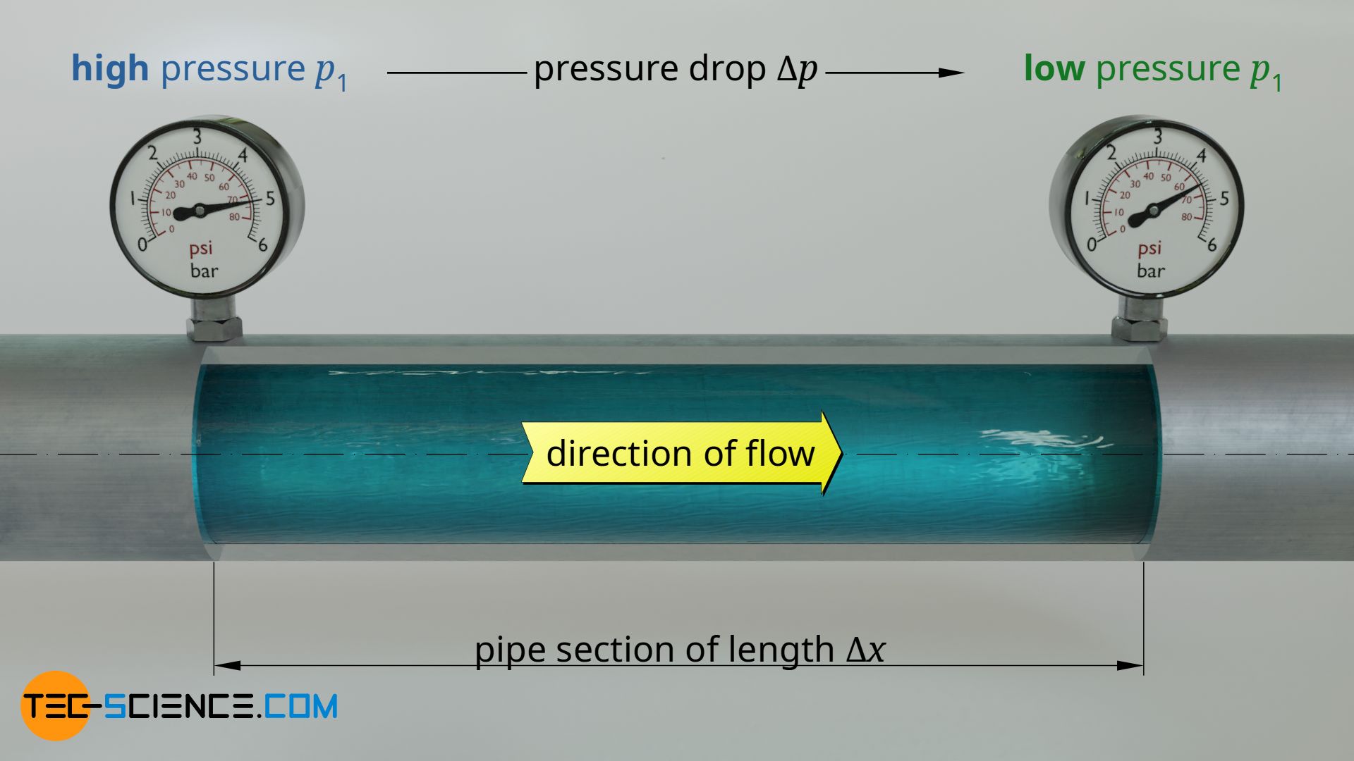
Flows are basically caused by pressure differences which push the fluid from points of higher pressure to points of lower pressure. A permanently decreasing pressure is thus formed along the pipe in the direction of flow. The greater this pressure drop over a certain length of the pipe, the faster the fluid flows through the pipe and the greater the flow rate. The drive for a flow is thus a pressure gradient dp/dx, i.e. the pressure drop per unit length.
Drive for flows in pipes are pressure gradients!
This drive is counteracted by frictional forces of the fluid, which act both between fluid and pipe and within the fluid itself. They are caused by the viscosity of the fluid.
Resistance for flows is caused by the viscosity of the fluid!
Laminar flows in pipes can be described mathematically on the basis of both forces, pressure forces as drive and friction forces as resistance. In the following, both the velocity profile and the volume flow rate of such a frictional pipe flow will be derived.
Derivation of the Hagen-Poiseuille equation
Pressure force acting on a volume element
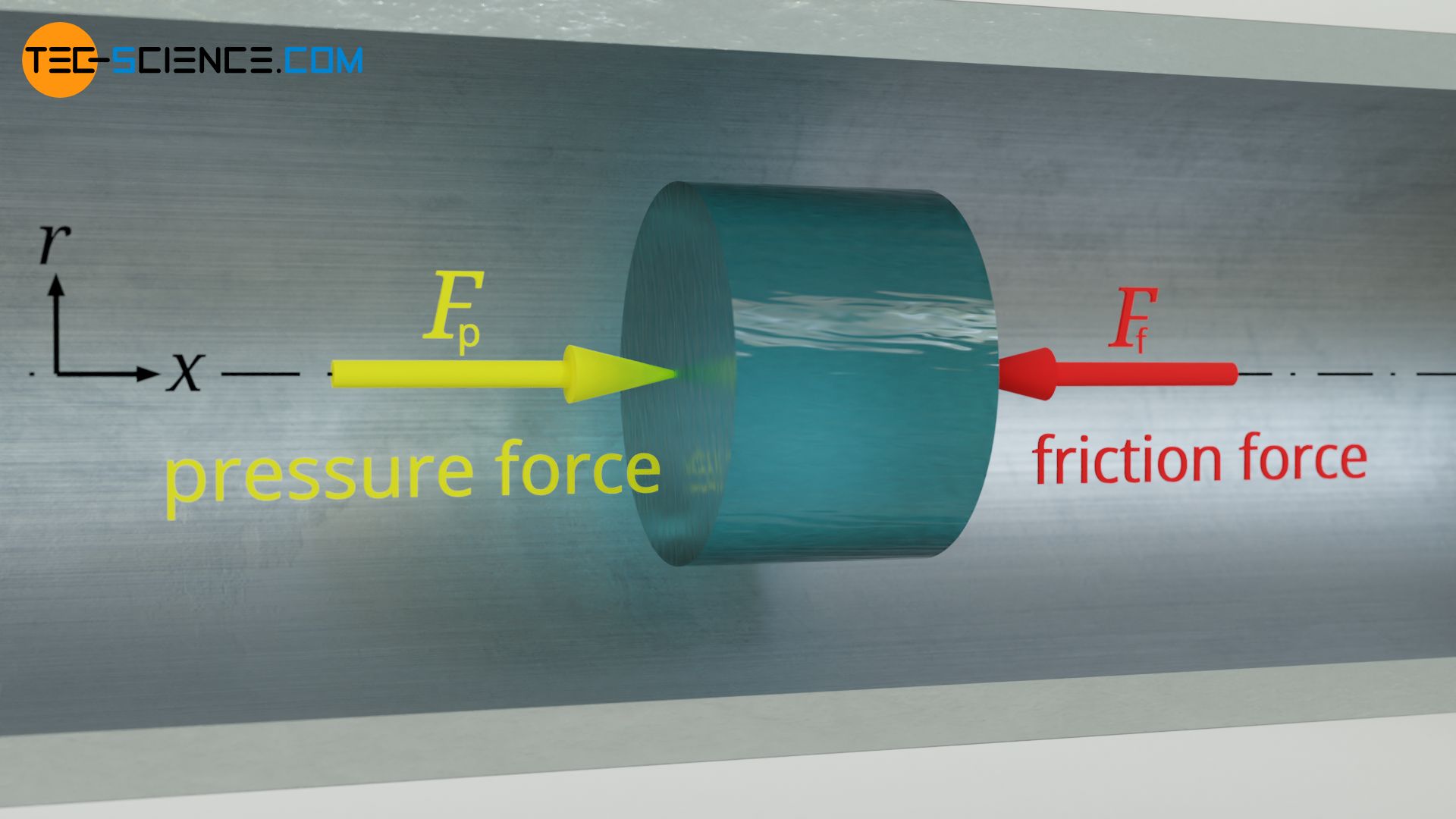
A cylindrical fluid element (fluid parcel) with the radius r is considered. Forces act on the end faces of this volume element which are considered constant over the entire cross-section of the pipe. These forces result from the pressures in the fluid acting on the faces of the volume element. At the point x1 the pressure p acts and at the point x2 a pressure lower by dp<0 acts. This results in the forces given below:
\begin{align}
&F_{\text{p}_1} = p \cdot \pi r^2 \\[5px]
&F_{\text{p}_2} = \left(p+\text{d} p\right) \cdot \pi r^2 \\[5px]
\end{align}
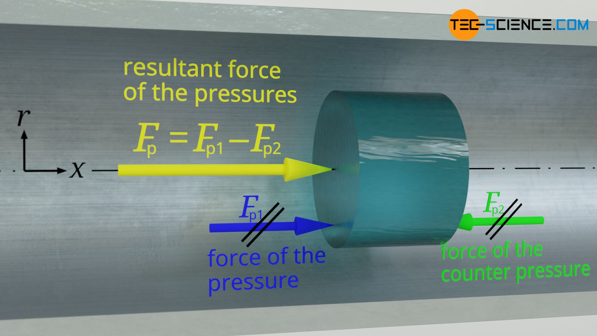
The resultant force Fp on the volume element with which the different pressures try to set the fluid in motion therefore results from the difference between the two forces:
\begin{align}
\require{cancel}
& F_\text{p}=F_{\text{p}_1} – F_{\text{p}_2} \\[5px]
& F_\text{p} = p \cdot \pi r^2 – \left(p+\text{d} p\right) \cdot \pi r^2 \\[5px]
& F_\text{p} = \cancel{p \cdot \pi \cdot r^2 } – \cancel{p \cdot \pi \cdot r^2 }- \text{d} p \cdot \pi r^2 \\[5px]
\label{fp}
&\boxed{ F_\text{p} = -\pi r^2 \cdot \text{d} p} \\[5px]
\end{align}
The driving force of the flow is therefore only due to the pressure drop (also called head loss) and not to the absolute pressures! Note that if the pressure is reduced along the positive axial direction, the pressure drop dp is negative, and the resultant force therefore acts along the positive axial direction.
Frictional force acting on a volume element (viscosity)
In principle, the speed of the flow within the pipe is not constant over the cross-section. There ist friction between the fluid and the pipe, which is why the flow velocity near the wall is lower than in the middle of the pipe. At the wall, the fluid even adheres to the wall due to the adhesive forces. Thus, there is no relative speed between fluid and wall. This is also called no-slip condition. But the individual fluid layers also have friction between each other due to the viscosity of the fluid. This leads to the formation of a certain velocity profile, the course of which is yet to be determined. It should be noted, however, that the flow velocity is maximum in the middle of the pipe and then drops to zero as far as the wall.
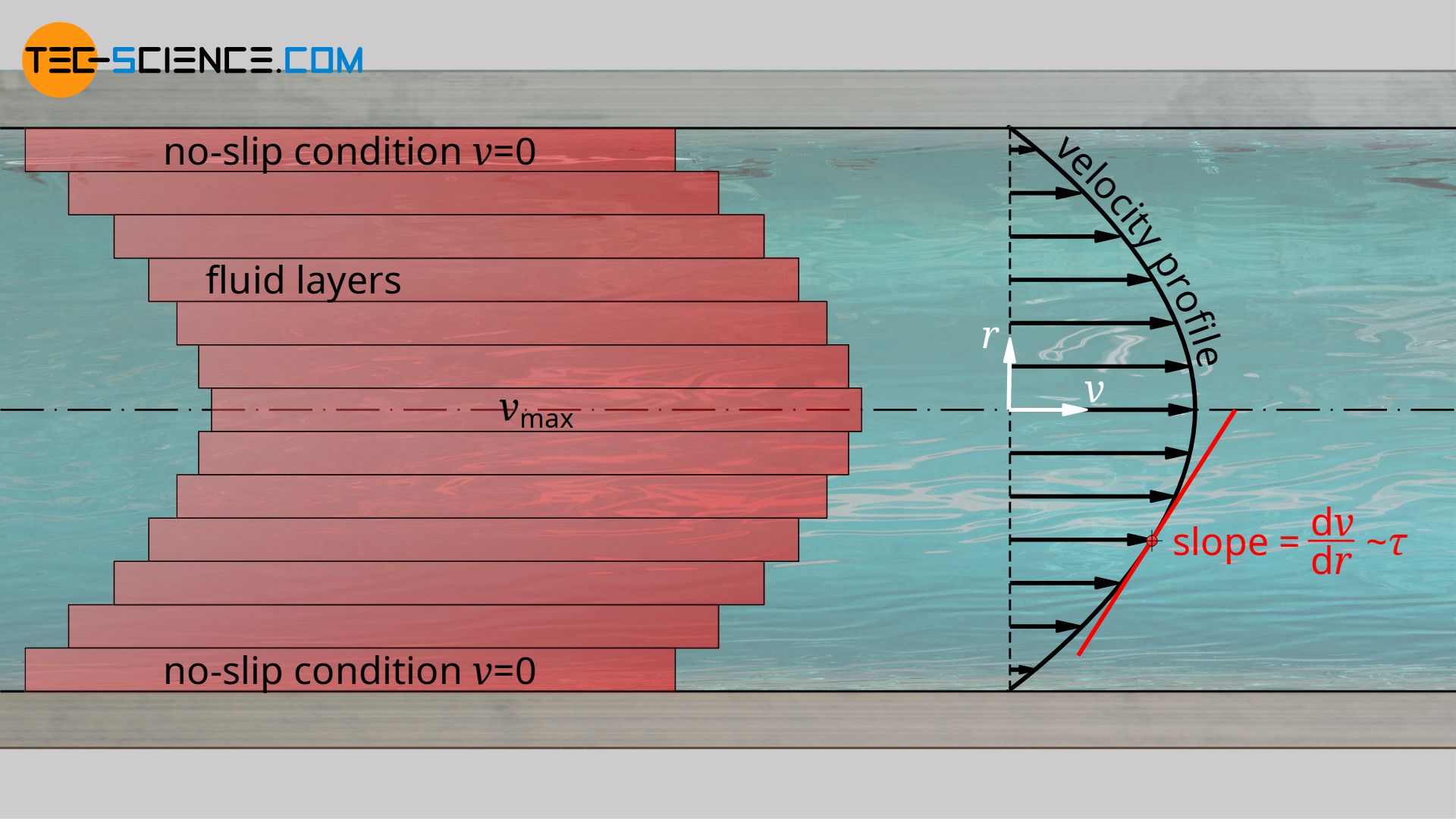
The flow resistance to be overcome, which is necessary to shear the individual fluid layers against each other, depends on the viscosity of the fluid. The flow resistance is expressed by the shear stress τ, i.e. as the force per unit area required to move a fluid layer. This shear stress depends on how much the fluid layers are displaced against each other. This in turn is expressed by the velocity gradient perpendicular to the flow direction, i.e. by the slope of the velocity profile in the radial direction dv(r)/dr (also called shear rate). The mathematical relationship between the two quantities is described by the viscosity η (Newton’s law of fluid motion):
\begin{align}
\label{vis}
&\boxed{\tau= \eta \cdot \frac{\text{d}v(r)}{\text{d}r}} \\[5px]
\label{sch}
&\boxed{\tau:=\frac{F}{A}} ~~~\text{ shear stress} \\[5px]
\end{align}
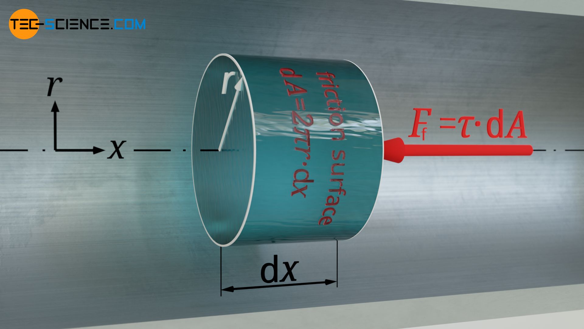
The driving force derived in the previous section due to the acting pressure forces is opposed by the frictional force between the considered volume element and the surrounding fluid. With τ as the area-related force, this frictional force Ff can be determined with the the area of the lateral surface of the cylindrical volume element 2π⋅r⋅dx. The shear stress τ is again given by the viscosity and the velocity gradient according to equation (\ref{vis}). Thus follows for the frictional force:
\begin{align}
& F_\text{f}=\tau \cdot \text{d}A = \tau \cdot 2 \pi r \cdot \text{d}x \\[5px]
\label{fr}
& \boxed{F_\text{f}= \eta \cdot \frac{\text{d}v(r)}{\text{d}r} \cdot 2 \pi r \cdot \text{d}x} \\[5px]
\end{align}
Velocity profile
For a steady flow, in which the flow velocities no longer change over time, a balance of forces applies to the volume element under consideration. The pressure force (\ref{fp}) and the counteracting frictional force (\ref{fr}) can thus be equated:
\begin{align}
\require{cancel}
& F_\text{f}= F_\text{p} \\[5px]
& \eta \cdot \frac{\text{d}v(r)}{\text{d}r} \cdot 2 \cancel{\pi r} \cdot \text{d}x = – \pi r^\cancel{2} \cdot \text{d} p \\[5px]
&\boxed{\frac{\text{d}v(r)}{\text{d}r}= – \frac{1}{2\eta} \frac{\text{d} p}{\text{d}x} \cdot r} \\[5px]
\end{align}
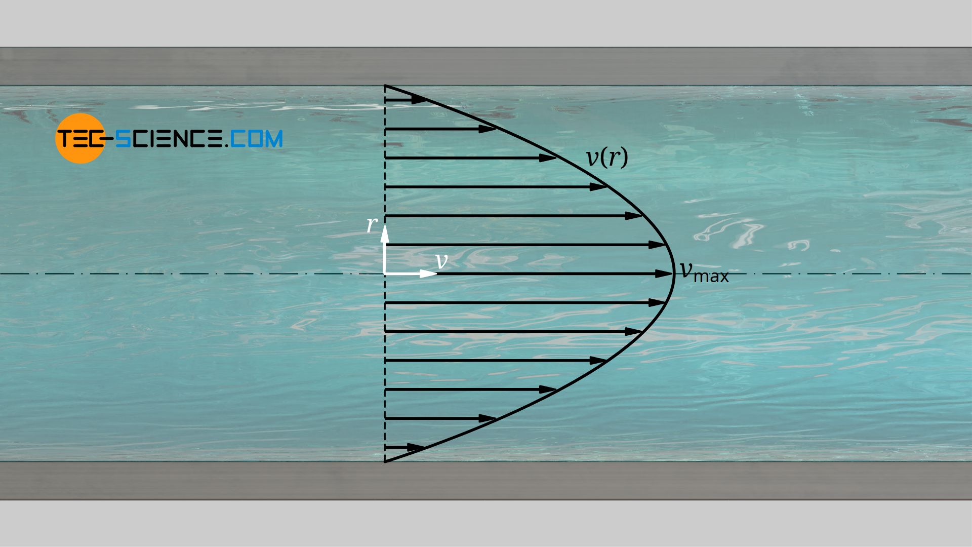
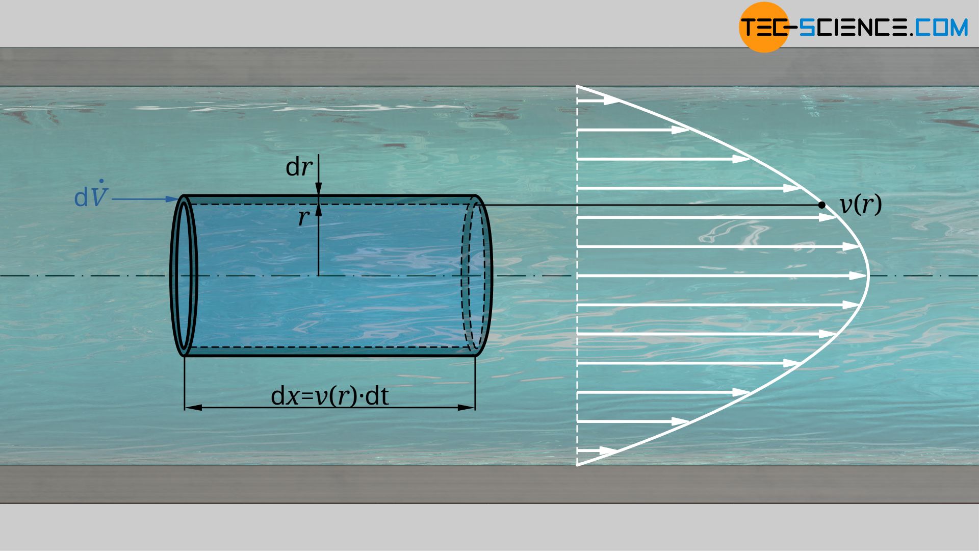
The left hand side of the equation denotes the velocity gradient of the flow in radial direction, i.e. the slope (derivative) of the velocity profile. On the right hand side is the pressure gradient in axial direction and the viscosity of the fluid. Both quantities are not a function of the radius. Therefore, the derivative of the velocity profile is a linear function. The actual velocity profile is therefore parabolic!
The exact velocity profile v(r) is obtained by integrating the above equation:
\begin{align}
&v(r)=\int -\frac{1}{2\eta} \frac{\text{d} p}{\text{d}x} \cdot r ~~\text{d}r \\[5px]
&v(r)=-\frac{1}{4\eta} \frac{\text{d} p}{\text{d}x} \cdot r^2 + C \\[5px]
\end{align}
The constant of integration C can be obtained from the boundary condition that the flow velocity at the pipe wall at r=R is zero (no-slip condition):
\begin{align}
&v(r=R)\overset{!}{=}0 \\[5px]
&-\frac{1}{4\eta} \frac{\text{d} p}{\text{d}x} \cdot R^2 + C = 0 \\[5px]
&\underline{C = \frac{1}{4\eta} \frac{\text{d} p}{\text{d}x} \cdot R^2} \\[5px]
\end{align}
If this constant is put into the above equation, the following velocity profile is finally obtained:
\begin{align}
&v(r)=-\frac{1}{4\eta} \frac{\text{d} p}{\text{d}x} \cdot r^2 +\frac{1}{4\eta} \frac{\text{d} p}{\text{d}x} \cdot R^2 \\[5px]
&v(r)=-\frac{1}{4\eta} \frac{\text{d} p}{\text{d}x} \cdot \left(R^2-r^2\right) \\[5px]
\label{vr}
&\boxed{v(r)=-\frac{R^2}{4\eta} \frac{\text{d} p}{\text{d}x} \cdot \left[1-\left(\frac{r}{R}\right)^2\right]} \\[5px]
\end{align}
Maximum flow velocity
The maximum flow velocity vmax is in the middle of the pipe. It can be determined by solving the above equation for r=0:
\begin{align}
&v_{\text{max}}=v(r=0) \\[5px]
&v_{\text{max}}= -\frac{R^2}{4\eta} \frac{\text{d} p}{\text{d}x} \cdot \left[1-\left(\frac{0}{R}\right)^2\right] \\[5px]
\label{max}
&\boxed{v_{\text{max}}= -\frac{R^2}{4\eta} \frac{\text{d} p}{\text{d}x} } \\[5px]
\end{align}
The maximum speed thus corresponds just to the expression before the rectangular brackets in equation (\ref{vr}), so that the velocity profile can also be represented with the following formula:
\begin{align}
\label{vrr}
&\boxed{v(r)=v_\text{max} \cdot \left[1-\left(\frac{r}{R}\right)^2\right]} ~~~\text{and}~~~\boxed{v_\text{max}=-\frac{R^2}{4\eta} \frac{\text{d} p}{\text{d}x}} \\[5px]
\end{align}
This equation, which states that the flow velocity increases parabolically from the wall to the centre of the pipe, is also known as the Hagen-Poiseuille equation. When deriving this equation, it was assumed that the viscosity is independent of the shear rate and thus not a function of the radius. Consequently, this equation only applies to so-called Newtonian fluids, where the viscosity is always constant. In addition, a laminar flow must be assumed for the validity of the equation, otherwise the viscosity loses its actual meaning.
Likewise, the Hagen-Poiseuille law loses its validity if the viscosity of the fluid is relatively low compared to the diameter of the pipe. This can also be clearly understood. For this purpose we imagine a pipe with a huge radius of e.g. 6 meters. Water flows through this pipe with a maximum flow velocity of e.g. 6 m/s. According to the Hagen-Poiseuille equation, at a distance of 10 cm from the wall a flow velocity of just 20 cm/s should be present. Experience already shows that the flow velocity at this relatively large distance from the pipe wall should be significantly higher (compare the flow velocity in a wide river, which is also almost maximum at a relatively small distance from the bank).
If, however, one would let much more viscous honey flow through the pipe in one’s thoughts, the relatively low flow velocity near the wall would suddenly no longer be so unrealistic. High viscosities influence the flow over the entire cross-section of the pipe, so to speak, while very low-viscosity fluids influence the flow only in a relatively small boundary area and no longer cover the entire cross-section (see also the article Boundary layers). To put it simply, the Hagen-Poiseuille law only applies if the viscosity is able to influence the entire flow cross-section. This assumes that the viscosity is not too low in relation to the diameter.
The Hagen-Poiseuille equation is the parabolic velocity profile of a frictional, laminar flow of Newtonian fluids in pipes whose lengths are large compared to their diameters! The flow itself is therefore also called Poiseuille flow.
Limitation of the Hagen-Poiseuille equation for short pipes
As already explained, a pressure drop between the beginning and the end of a pipe is the drive for a flow. However, the pressure gradient that forms over the length of the pipe has two tasks, so to speak. The pressure drop must not only compensate the frictional force during the flow of the fluid, but must accelerate the fluid to achieve the characteristic flow profile in the first place.
Therefore, the total pressure drop can be divided into a part which is used to accelerate the fluid and a part which is used to compensate for friction. As already explained at the beginning, in the above equations, the pressure gradient dp/dx only refers to that part of the total pressure gradient which is necessary to overcome the friction.
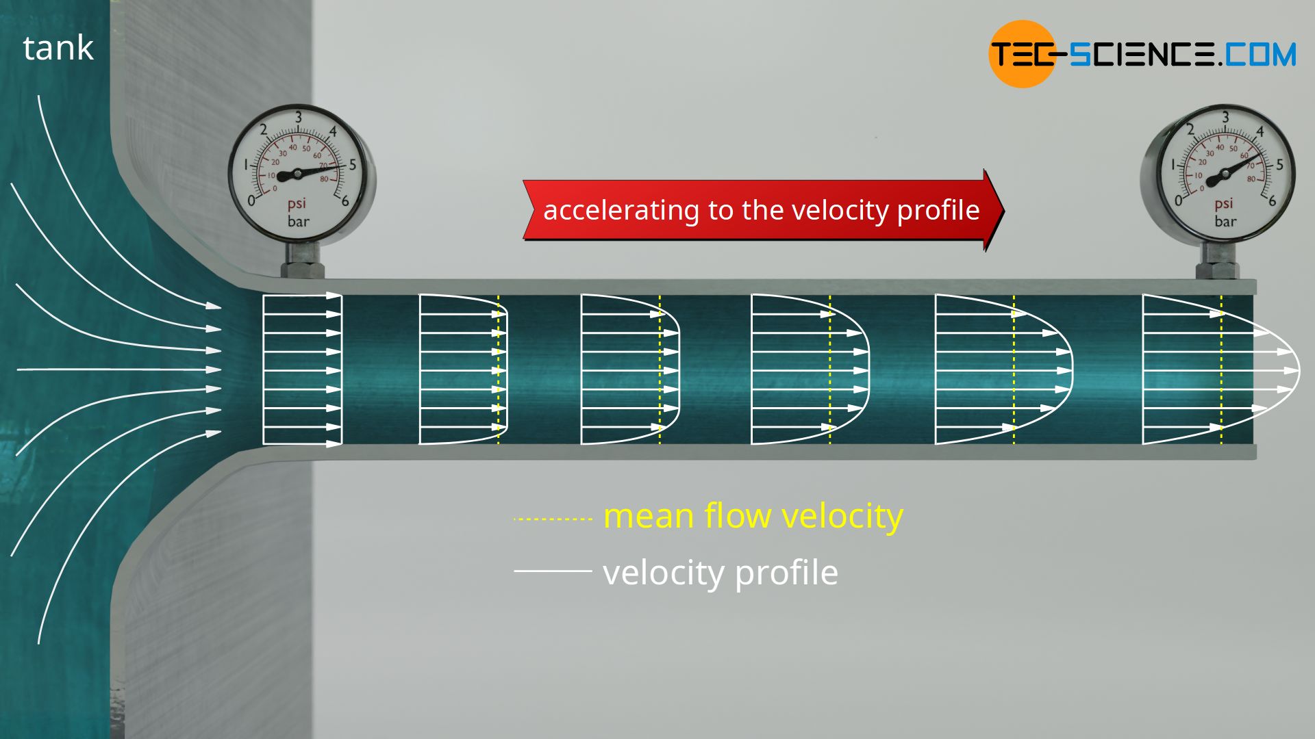
To determine this pressure gradient, one must not simply take the pressure difference between the beginning and end of the pipe and then divide it by the length of the pipe. This is why the above equations always referred to a pipe section where it was implicitly assumed that the parabolic flow profile had already been fully established.
The equation of Hagen-Poiseuille does not apply in the inlet of a pipe (inlet flow), within which the pressure gradient must accelerate the fluid to the typical parabolic profile in addition to overcoming friction!
Under certain circumstances, it may nevertheless be justified to describe flow by simply determining the pressure gradient in the above equations from the quotient of pressure drop and pipe length. Namely, whenever the work of acceleration is negligible compared to the friction work. This will always be the case if the pipe is relatively long compared to its diameter, or if the flow velocities are relatively low. In such cases, the frictional work usually clearly outweighs the relatively low work of acceleration due to the long pipe length.
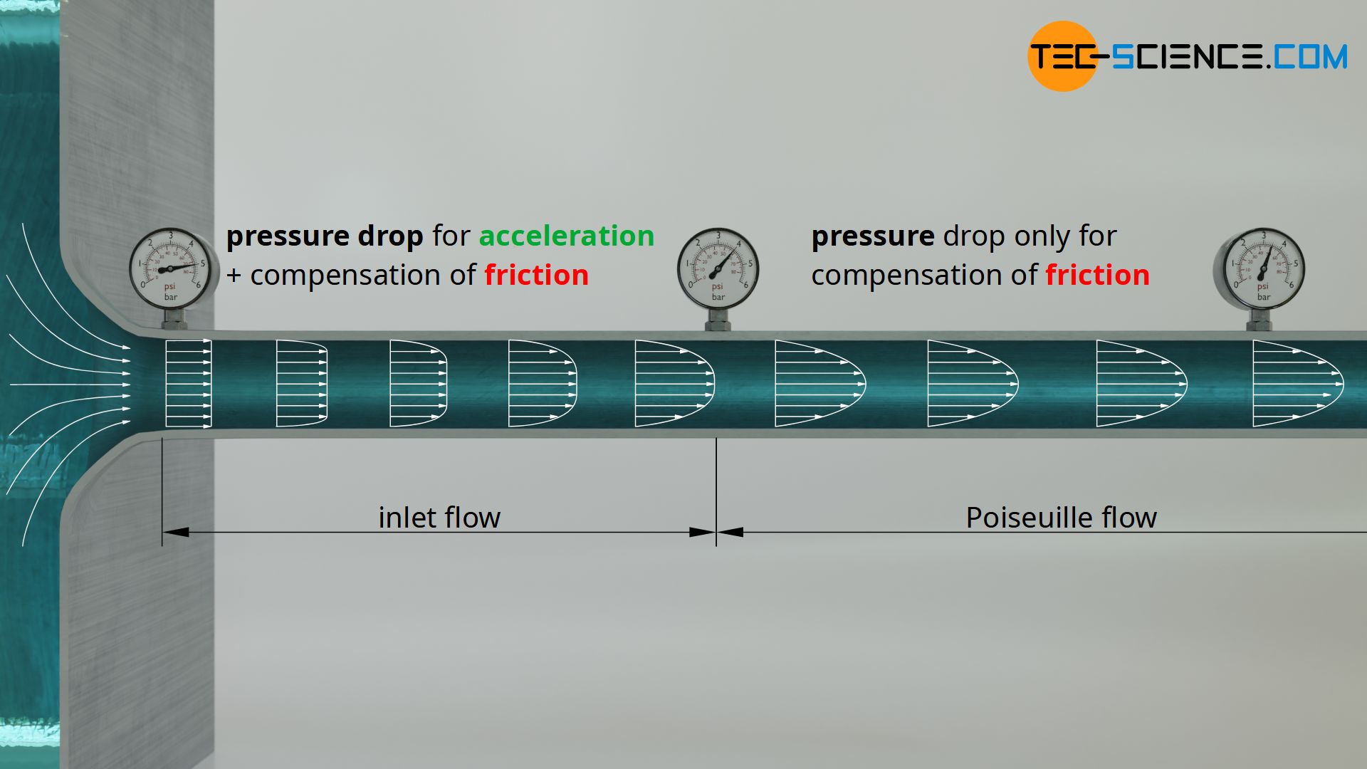
However, with relatively short pipes, the part of the pressure drop required to accelerate the fluid is no longer negligible. In such a case, the parabolic velocity profile cannot fully develop within the short pipe. The Hagen-Poiseuille equation is no longer valid in this case (no parabolic velocity profile)! More information on this topic can be found in the article Energetic analysis of the Hagen-Poiseuille Law.
The Hagen-Poiseuille equation is only valid for long pipes whose length is relatively large compared to their diameter.
Volume flow rate
Since the velocity profile is now known, the volume flow rate can now be determined by the cross-section of a pipe. To derive the flow rate, we consider a ring with the infinitesimal thickness dr at any distance r from the center of the pipe . The area of the considered ring dA can be derived from the “length” of the ring 2π⋅r (circumference) and the “height” of the ring dr (thickness):
\begin{align}
\label{q}
&\text{d}A = 2\pi r \cdot \text{d}r \\[5px]
\end{align}
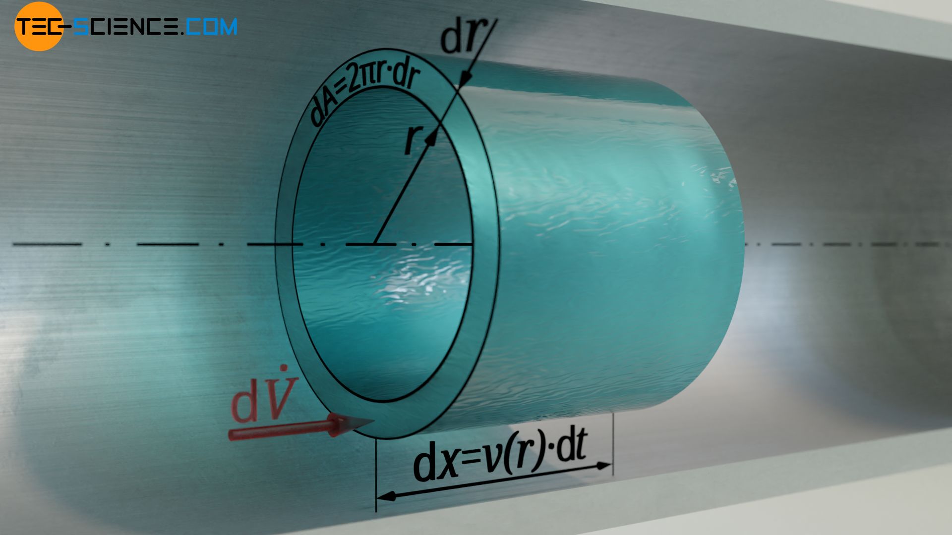
The speed at which the fluid flows through this ring at the distance r is given by equation (\ref{vr}). Within the time dt, the fluid covers the distance dx=v(r)⋅dt. Thus, the liquid takes up a volume dV which results in the following flow rate dV*:
\begin{align}
&\text{d}V = \text{d}A \cdot \text{d}x = 2\pi r \cdot \text{d}r \cdot v(r) \cdot \text{d}t \\[5px]
&\text{d}V = -2\pi r \cdot \frac{R^2}{4\eta} \frac{\text{d} p}{\text{d}x} \cdot \left[1-\left(\frac{r}{R}\right)^2\right] \cdot \text{d}r \cdot \text{d}t \\[5px]
&\text{d}\dot V = \frac{\text{d}V}{\text{d}t} = – \frac{ 2\pi R^2}{4\eta} \frac{\text{d} p}{\text{d}x} \cdot \left[r-\frac{r^3}{R^2}\right] \cdot \text{d}r \\[5px]
\end{align}
The volume flow rate V* through the entire pipe is finally obtained by integrating this equation with respects to the radius r within the limits from r=0 to r=R:
\begin{align}
&\dot V = \int\limits_{(A)}^{} \text{d} \dot V = \int\limits_0^R – \frac{ 2\pi R^2}{4\eta} \frac{\text{d} p}{\text{d}x} \cdot \left[r-\frac{r^3}{R^2}\right] \cdot \text{d}r \\[5px]
&\dot V = – \frac{ 2\pi R^2}{4\eta} \frac{\text{d} p}{\text{d}x} \cdot \left\vert \frac{r^2}{2}-\frac{r^4}{4R^2}\right\vert_0^R \\[5px]
&\dot V = – \frac{ 2\pi R^2}{4\eta} \frac{\text{d} p}{\text{d}x} \cdot \left(\frac{R^2}{2}-\frac{R^4}{4R^2}\right) = – \frac{ 2\pi R^2}{4\eta} \frac{\text{d} p}{\text{d}x} \cdot \frac{R^2}{4} \\[5px] \\[5px]
\label{dv}
&\boxed{\dot V = – \frac{\pi R^4}{8\eta} \frac{\text{d} p}{\text{d}x} } \\[5px]
\end{align}
What is particularly remarkable about this result is that the pipe radius influences the flow rate with the fourth power. A doubling of the pipe radius therefore means a 16-fold volume flow! Note that this relationship only applies to incompressible fluids whose volume does not change with pressure. As before, a laminar flow of a Newtonian fluid must be assumed.
The equation of the flow rate have a further meaning in practice. The flow rate is directly dependent on the viscosity of the fluid. The viscosity of a fluid can therefore be easily determined from the flow rate. A capillary viscometer is based on this principle.
Remark
Frequently, reference is made at this point to the example of the narrowing of veins and fine blood vessels, which according to the formula of the flow rate would indeed have enormous effects on the blood flow and the required blood pressure. In this context, however, blood is rather an inappropriate example, even though Poiseuille actually took the flow of blood as an occasion to investigate such flows more closely.
Blood is not a Newtonian fluid, but a shear-thinning (pseudoplastic) fluid. And especially in the case of very fine blood vessels or in the case of a narrowing, the flow profile is quite the opposite of a Poiseuille flow! In very fine vessels, the blood cells move like large plugs with an almost constant flow velocity over the entire cross-section. This is also called plug flow.
Furthermore, turbulent flows can occur at narrowings and high flow velocities, which would then also lead to an almost constant velocity profile (see section on turbulent flow).
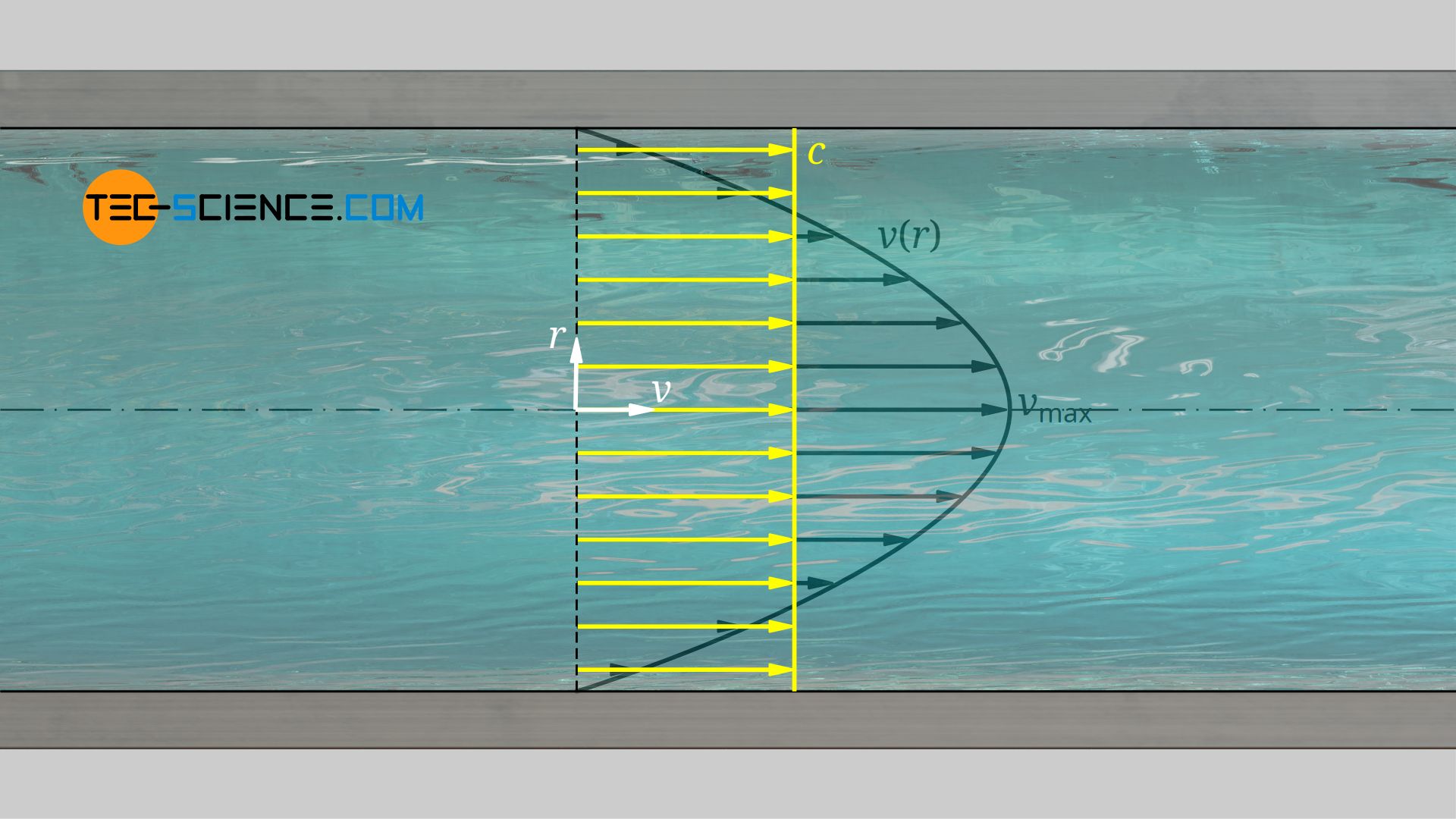
Mean flow velocity
With its parabolic velocity profile, a flow inside a pipe has no characteristic velocity in principle. Therefore, a mean flow velocity c is often defined to characterize such flows. The mean flow velocity is defined as a constant velocity over the entire cross-section which provides the same flow rate as the real velocity profile. With A=π⋅R2 as the inner pipe cross section, the mean flow velocity c can be determined by the volume flow rate V*:
\begin{align}
\label{dvv}
&\dot V = \frac{\Delta V}{\Delta t} = \frac{A \cdot \Delta x}{\Delta t} = \pi R^2 \cdot \frac{\Delta x}{\Delta t} = \pi R^2 \cdot c \\[5px]
\end{align}
In the above derivation it was used that the quotient of traveled distance Δx and time Δt just corresponds to the mean flow velocity. Equating the equations (\ref{dvv}) and (\ref{dv}) finally provides the mean flow velocity c:
\begin{align}
&\pi R^2 \cdot c =- \frac{\pi R^4}{8\eta} \frac{\text{d} p}{\text{d}x} \\[5px]
\label{c}
& \boxed{c =- \frac{R^2}{8\eta} \frac{\text{d} p}{\text{d}x}} ~~~\text{mean flow velocity}\\[5px]
\end{align}
The following relationship applies between the maximum flow velocity vmax and the mean flow velocity c:
\begin{align}
&\frac{c}{v_\text{max}} = \frac{ – \frac{R^2}{8\eta} \frac{\text{d} p}{\text{d}x} }{ -\frac{R^2}{4\eta} \frac{\text{d} p}{\text{d}x} } = \frac{1}{2}\\[5px]
&\boxed{c = \frac{1}{2} \cdot v_\text{max}}
\end{align}
The mean flow velocity is half the maximum flow velocity in the middle of the pipe!
Pressure loss
As already explained, the pressure gradient dp/dx in the upper equations represents the drive for the flow of the fluid. According to the equation (\ref{dv}), this directly influences the flow rate. Conversely, this means that a pressure gradient must exist for a desired flow rate. This requires a pump which ultimately generates this pressure gradient (at this point the negative sign is omitted, since only the amounts are decisive anyway):
\begin{align}
& \frac{\text{d} p}{\text{d}x} = \frac{8\eta}{\pi R^4} \dot V \\[5px]
\end{align}
From the definition of the pressure gradient as change in pressure per unit length, the pressure drop Δpd required over a pipe section with the length ΔL can be calculated with the following formula:
\begin{align}
\label{pv}
& \frac{\text{d}p}{\text{d}x} = \frac{\Delta p_d}{L} \\[5px]
& \Delta p_d = \frac{\text{d}p}{\text{d}x} \cdot \Delta L \\[5px]
& \underline{\Delta p_d = \frac{8\eta \cdot \Delta L}{\pi R^4} \dot V } \\[5px]
\end{align}
For a friction-free flow, on the other hand, no such pressure drop would have to be applied in the steady state to keep the fluid flowing. Once set in motion, the fluid would flow through the pipe without loss of speed. The application of the pressure is therefore due to the friction loss, which is equivalent to a pressure drop. In the steady case, the pressure created by a pump must fully compensate for the pressure loss in order to keep the fluid flowing. The above formula is therefore equivalent to the pressure loss Δpl, which occurs over the pipe length ΔL:
\begin{align}
& \boxed{\Delta p_l = \frac{8\eta \cdot \Delta L}{\pi R^4} \dot V} ~~~\text{pressure loss} \\[5px]
\end{align}
You can illustrate the situation by looking at a pipe through which a foam rod is to be pressed. To push it through, the frictional force between the foam and the pipe must be overcome. A certain force is required for this. However, the force applied from this side of the pipe does not correspond to the force that a second person at the end of the pipe perceives. This person thus measures a much lower force.
Thus, a loss of force occurs towards the end of the pipeline, which is the greater the greater the friction and thus the pipeline is. If one relates the force to the cross-sectional area of the pipe, this ultimately corresponds to a pressure. So there is a pressure loss along the pipe. In the steady case at a constant speed, there is a balance of forces, so that the pressure loss Δpl due to the frictional force just corresponds to the pressure difference Δpd between the beginning and end of the pipe with which the foam is pushed through.
The volume flow rate in the upper equation can also be expressed by the mean flow velocity according to equation (\ref{c}). The pressure loss as a function of the mean flow velocity is thus:
\begin{align}
& \Delta p_l = \frac{8\eta \cdot \Delta L}{\pi R^4} \cdot \overbrace{\pi R^2 \cdot c}^{\dot V} \\[5px]
& \boxed{\Delta p_l = \frac{8\eta \cdot \Delta L}{R^2} \cdot c} ~~~\text{pressure loss} \\[5px]
\end{align}
The pressure loss along a pipe is proportional to the mean flow velocity in laminar flow! This relationship no longer applies to turbulent flows.
Note that the pressure loss described is based purely on viscosity (“viscous pressure loss”). This pressure loss must always be applied by a pump to keep the fluid flowing. Pressure losses that occur, for example, due to pipe angles are not taken into account by the formulas above. However, the equations show that the pipe radius obviously has a great influence on the pressure loss. Large pipes generally lead to a lower (viscous) pressure loss. By using large pipes, the mechanical power of the pump P can therefore be significantly reduced for the same volumetric flow rate V*:
\begin{align}
& P = \Delta p_l \cdot \dot V = \frac{8\eta \cdot \Delta L}{\pi R^4} \dot V^2\\[5px]
& \boxed{P = \frac{8\eta \cdot \Delta L}{\pi R^4} \dot V^2}\\[5px]
\end{align}
Velocity profile for turbulent flows
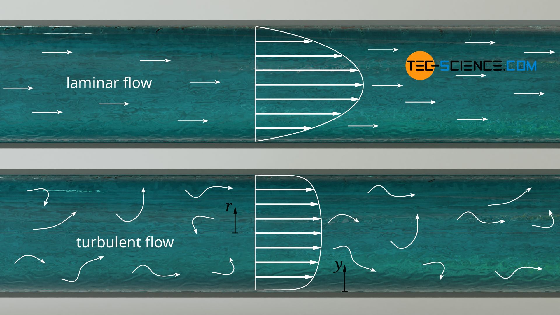
A parabolic velocity profile is only formed in pipes if a laminar flow is present. If the flow would change into a turbulent flow under otherwise identical conditions, the maximum flow velocity in the pipe center is lower due to the turbulence. At the same time, however, the increased mixing due to the turbulent flows leads to a stronger transfer of momentum between the fluid particles, so that the flow velocity increases stronger in the area close to the wall. For turbulent flows with Reynolds numbers greater than about 2300, the following approach is therefore often used to describe the velocity profile with a so-called a flow index n:
\begin{align}
&\boxed{v(r)=v_\text{max} \cdot \left(1-\frac{r}{R}\right)^\frac{1}{n}} ~~~\text{turbulent flow}\\[5px]
\end{align}
The following function applies to a coordinate system whose origin is the pipe wall:
\begin{align}
&\boxed{v(z)=v_\text{max} \cdot \left(\frac{y}{R}\right)^\frac{1}{n}} ~~~~0<y<R\\[5px]
\end{align}
In practice, n=7 is often chosen for the flow index. This is also known as the 1/7-power-law (one-seventh power law). In this case, the following relationship applies between the mean and the maximum flow velocity:
\begin{align}
&\boxed{c = 0.817 \cdot v_\text{max}} ~~~\text{for } n=7\\[5px]
\end{align}
The flow index depends on the Reynolds number and on the relative roughness of the pipe wall, i.e. the ratio between surface roughness and diameter of the pipe.
Remark: The 1/7-power-law is also used, for example, to describe turbulent boundary layers. After all, the entire pipe flow is a single large boundary layer.
")


")
")
