In this article you can learn more about the experimental determination of the thermal conductivity of materials using steam and ice.
Thermal conductivity
Thermal conductivity is a measure of how well or poorly a material conducts heat. The thermal conductivity λ describes the relationship between a temperature gradient ΔT along a distance Δx and the resulting rate of heat flow Q* through the area A:
\begin{align}
&\boxed{\dot Q =\lambda \cdot A \cdot \frac{\Delta T}{\Delta x}} ~~~~~\text{and}~~~~~[\lambda]=\frac{\text{W}}{\text{m} \cdot \text{K}} ~~~~~\text{thermal conductivity}\\[5px]
\end{align}
Detailed information about this equation, also known as Fourier’s law, can be found in the article on Thermal conductivity. In this article we will only focus on the experimental determination of thermal conductivity, which is based on the equation above:
\begin{align}
\label{a}
&\boxed{\lambda =\frac{\dot Q \cdot \Delta x}{\Delta T \cdot A}}
\end{align}
In order to determine the thermal conductivity λ of a material with a thickness Δx and an area A, a temperature difference ΔT must first be applied and the resulting heat flow rate Q* must be determined.
Principle of measurement
In the following a relatively simple experiment will be presented with which the thermal conductivity of a material sample can be determined.
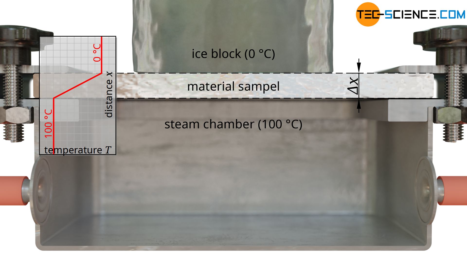
For this purpose, a slab-shaped sample is used, for whose material the thermal conductivity is to be determined. In the case shown, it is a metal plate. This metal plate has the thickness Δx = 10 mm and is heated from one side and cooled from the other. The figures below show the experimental setup.
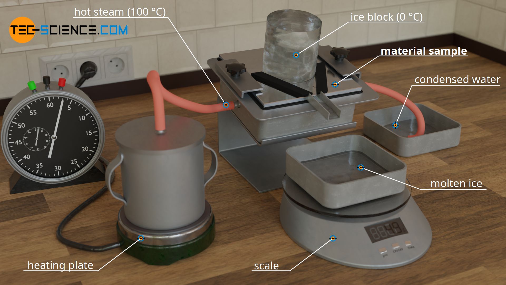
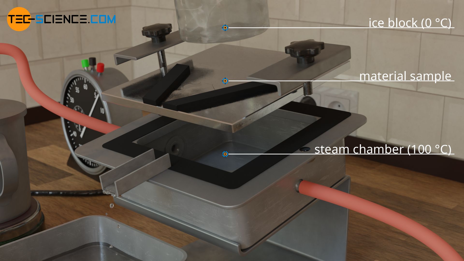
Heating is done with hot steam, which generates a temperature of exactly 100 °C when condensing on the plate. For temperature control of the cold side, a block of ice is used, which creates a temperature of exactly 0 °C on the plate during melting. This results in a temperature drop of ΔT = 100 °C along the thickness of the plate.
The rate of heat flow is determined by the amount of melted water. For this purpose, the melted water within a certain time is collected and weighed. Using the specific heat of fusion of the ice of qf=334 kJ/kg and the melted water mass m within the time Δt, the heat flow rate Q* through the sample plate is determined as follows:
\begin{align}
&\dot Q=\frac{Q}{\Delta t} = \frac{q_s \cdot m}{\Delta t}
\end{align}
If, for example, an ice mass of m = 50 g melts within the time Δt = 17 s, then according to the upper formula a heat flow rate of Q* = 982 J/s results.
However, the timing and collection of the melted water must not be started immediately after the ice block has been put on the specimen. First of all, a steady state must be established, i.e. you have to wait some time until the temperatures in the material do not change any more and a temperature gradient that is constant over time has been established. The thermal conductivity only refers to such steady states where the rate of heat flow is constant in time. The change of temperature while the sample is still warming up, however, is described by the so-called thermal diffusivity (although both quantities are linked together). This temperature propagation is a so-called unsteady state in which the rate of heat flow is not constant in time. In the simulation below the steady state is reached after about 10 seconds.
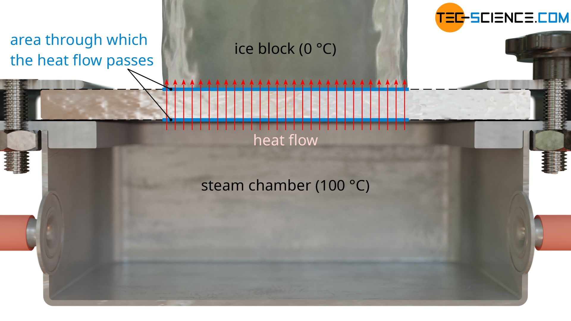
As a further quantity for calculating the thermal conductivity, the area A through which the heat flow passes is also required. This corresponds to the contact surface of the ice block. Note: Not the entire surface of the plate may be used as a basis, since the heat flow relevant for melting the ice block only passes through the area where the ice block is located. The heat flows outside of this area, which are considered one-dimensional, are transferred to the air and are not taken into account by the melting process (more about this later).
With a diameter of the ice block of e.g. 5 cm, this results in a area of A = 0.00196 m².
Now that all relevant parameters have been determined (sample thickness, temperature drop, area and heat flow rate), the thermal conductivity of the material sample used can finally be determined according to equation (\ref{a}). With these given values one obtains a thermal conductivity of λ= 50 W/(m⋅K).
\begin{align}
&\lambda =\frac{\dot Q \cdot \Delta x}{\Delta T \cdot A} = \frac{982 \frac{\text{J}}{\text{s}} \cdot 0.01 \text{ m}}{100 \text{ K} \cdot 0.00196 \text{ m²}} = 50 \frac{\text{W}}{\text{m}\cdot \text{K}}
\end{align}
Cons of this experimental setup
No pure thermal conduction
When determining thermal conductivity experimentally, it should be noted that thermal conductivity by definition only refers to heat transfer by thermal conduction, not convection or radiation! In the case of materials containing gases (e.g. autoclaved aerated concrete), however, thermal convection in the gas pores cannot be avoided. Heat radiation can also penetrate the material under certain circumstances. These heat transfer mechanisms are (unintentionally) taken into account in the experimental determination of thermal conductivity. However, the influence of thermal radiation can be minimized if the sample is as thick as possible so that radiation hardly penetrates the sample. However, this has another disadvantage, as will be shown in a moment.
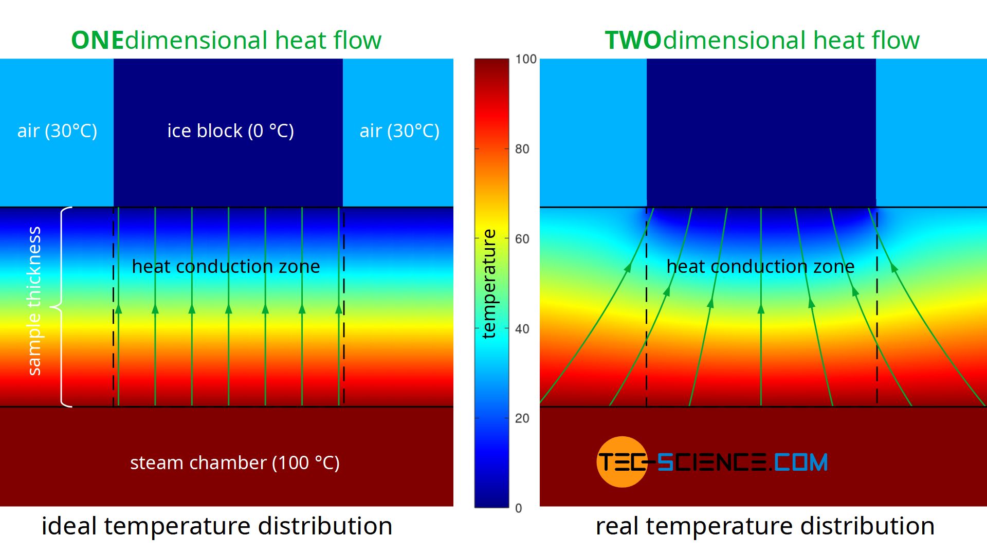
No one-dimensional heat flow
A further disadvantage of the experiment described is that during the performance of the experiment there is no one-dimensional heat flow through the material, as Fourier’s law requires on a macroscopic scale. Heat, so to speak, does not flow straight through the sample, but also enters the heat conduction zone (measuring zone) laterally. The heat flow is therefore based on a larger surface area on the hot underside of the sample than on the upper side where the ice block is located (see figure below). This effect of the two-dimensional heat flow has less influence on the result, the thinner the sample material is in comparison to the surface. At the same time, however, the influence of thermal radiation increases, since this penetrates thin samples more strongly than thick ones.
The figure below shows the simplified simulation of the temperature distribution and thus the heat flow. Modelling was done with a constant temperature at the bottom of the plate and constant temperatures at the top. The temperatures towards the ice block and towards the environment were assumed to be sharply limited. The simulation shows the formation of a two-dimensional heat flow as it occurs in reality. In comparison, the figure also shows a one-dimensional heat flow as it is actually required for the Fourier’s law to be valid.
Temperature dependence of thermal conductivity
Another disadvantage of the described method refers to the adjustment of the temperatures. Strictly speaking, the thermal conductivity is not a material constant, but depends on the temperature. The method therefore only measures an average thermal conductivity in the range between 0 °C and 100 °C. A more detailed investigation of the thermal conductivity as a function of temperature is not possible with such a experimental setup. The temperatures are fixed when using steam and ice and cannot be changed.
Generating one-dimensional heat flows
For the determination of the thermal conductivity according to equation (\ref{a}) to be valid at all, a one-dimensional heat flow must be ensured. This can be achieved, for example, by controlling the temperature outside the actual heat conduction zone (measuring zone). The temperature is chosen identically to the temperature of the cooled side. Therefore the sample plate around the ice block is also brought to a temperature of 0 °C.
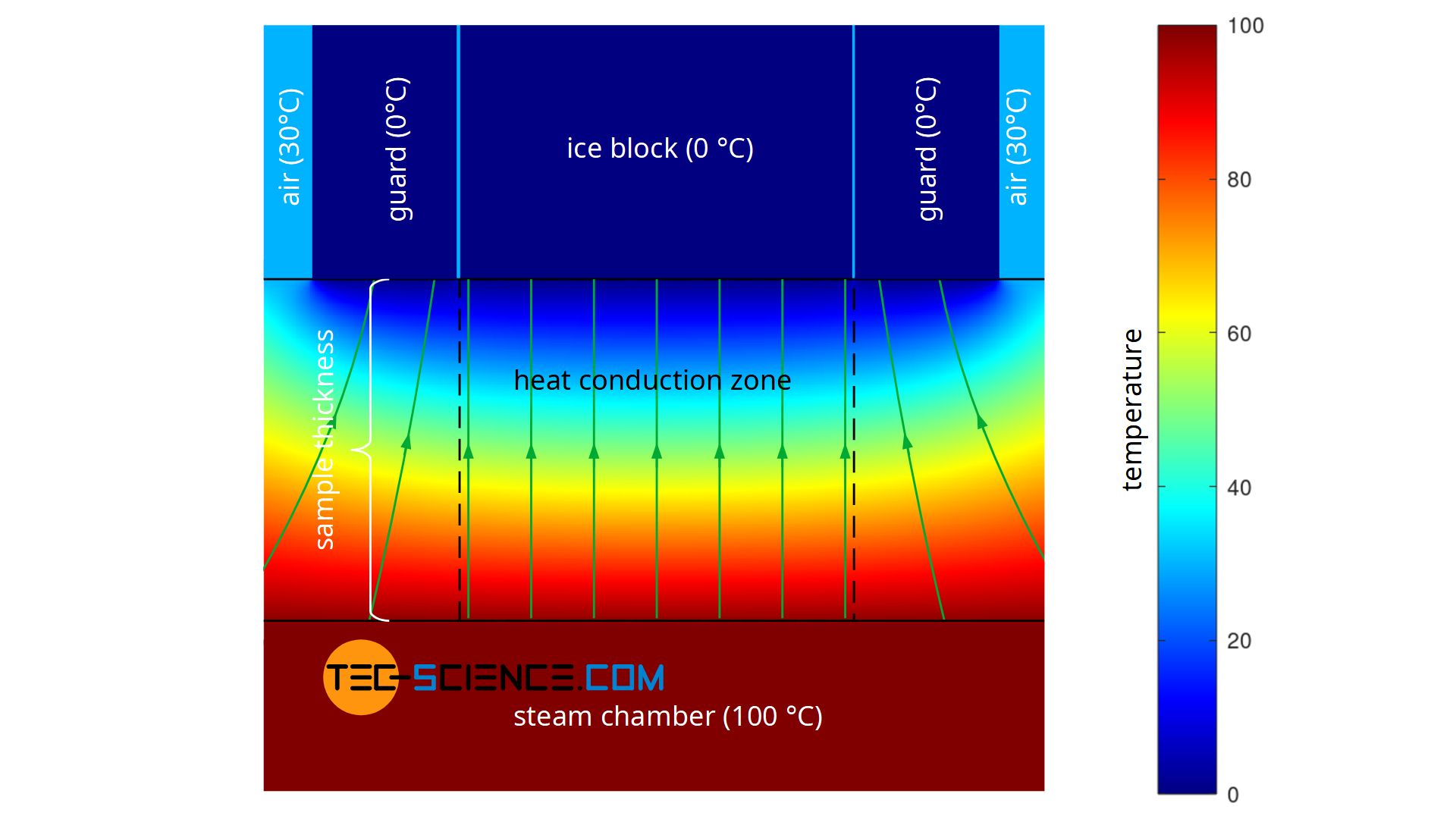
Of course, a ring of ice cannot be used here, because it would also melt and thus be taken into account in the calculation of the thermal conductivity. This would only have enlarged the original ice block. The two-dimensional heat flows at the edges of the heat conduction zone would still remain. However, a metal ring could be placed around the ice block and cooled to a temperature of 0 °C. In this way, the two-dimensional heat flow would be shifted close to the metal ring and provide an almost one-dimensional heat flow within the actual measuring zone.
Such a temperature-controlled ring, which guides the heat flow in a one-dimensional direction, is also known as a guard ring (guard for short). This principle of a guided heat flow is used, for example, in the so-called Guarded-Hot-Plate Method (GHP), which is described in more detail in the linked article.
")


")

