The heat equation describes the temporal and spatial behavior of temperature for heat transport by thermal conduction.
Derivation of the heat equation
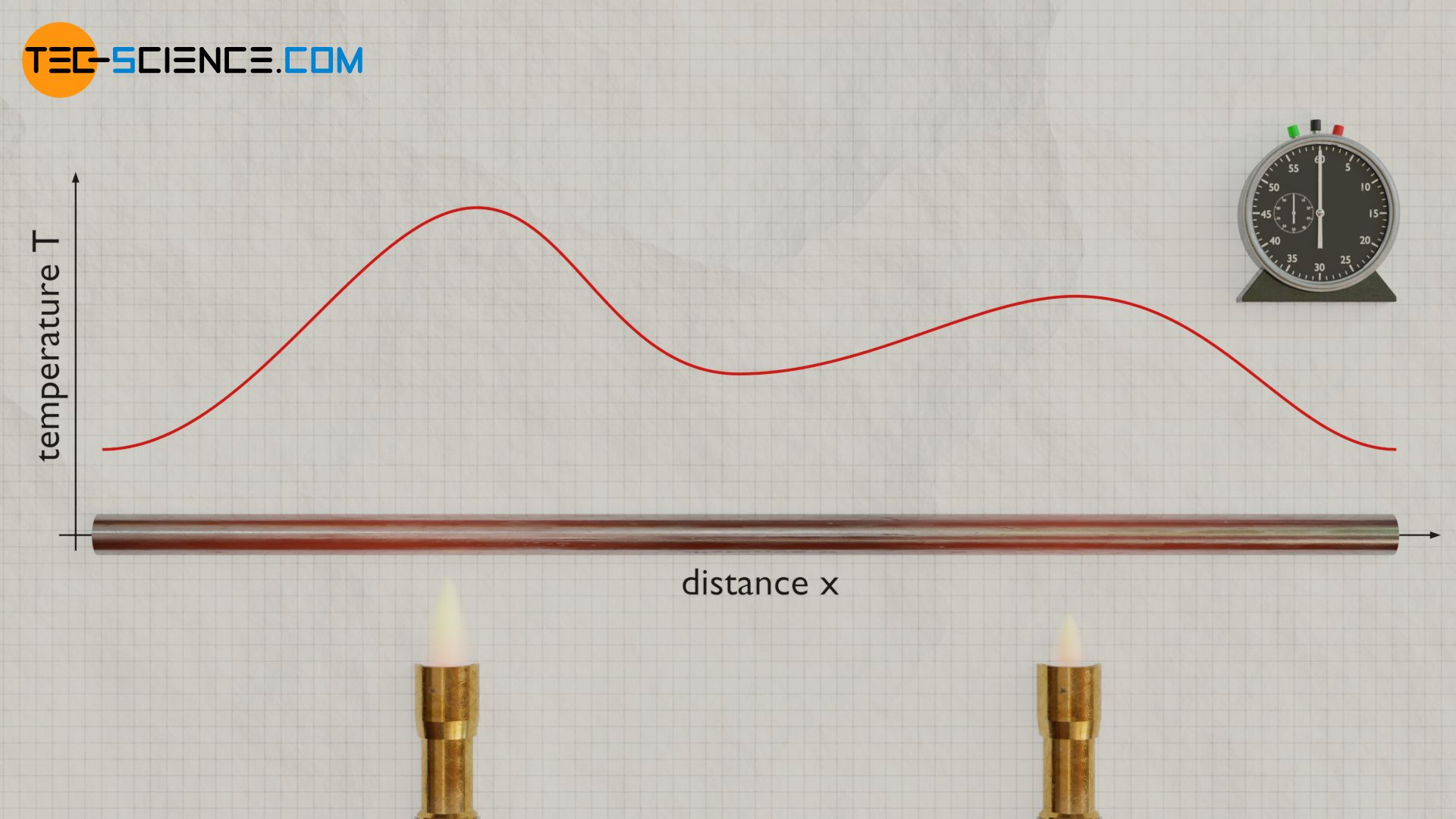
We first consider the one-dimensional case of heat conduction. This can be achieved with a long thin rod in very good approximation. We assume that heat is only transferred along the rod and not laterally to the surroundings (thermally-insulated rod).

In addition, the material properties of the homogeneous rod, such as heat capacity and density, are considered to be constant. Now the rod is heated at one point or even at several points. Heat then flows from places of higher temperature to places with lower temperatures. As a result, hot spots become colder and cooler spots hotter, until at some point the temperatures have equalized and the rod has a uniform and temporally constant temperature.
During temperature equalization we now consider an infinitesimal section dx at any point. This section changes its temperature by dT within the time period dt due to the heat Qn. The following relationship applies between the heat Qn and the temperature change dT (c denotes the specific heat capacity):
\begin{align}
&Q_n = m \cdot c \cdot \text{d}T \\[5px]
&Q_n = \underbrace{\overbrace{A \cdot \text{d}x}^{V} \cdot \rho}_{m} \cdot c \cdot \text{d}T \\[5px]
\end{align}
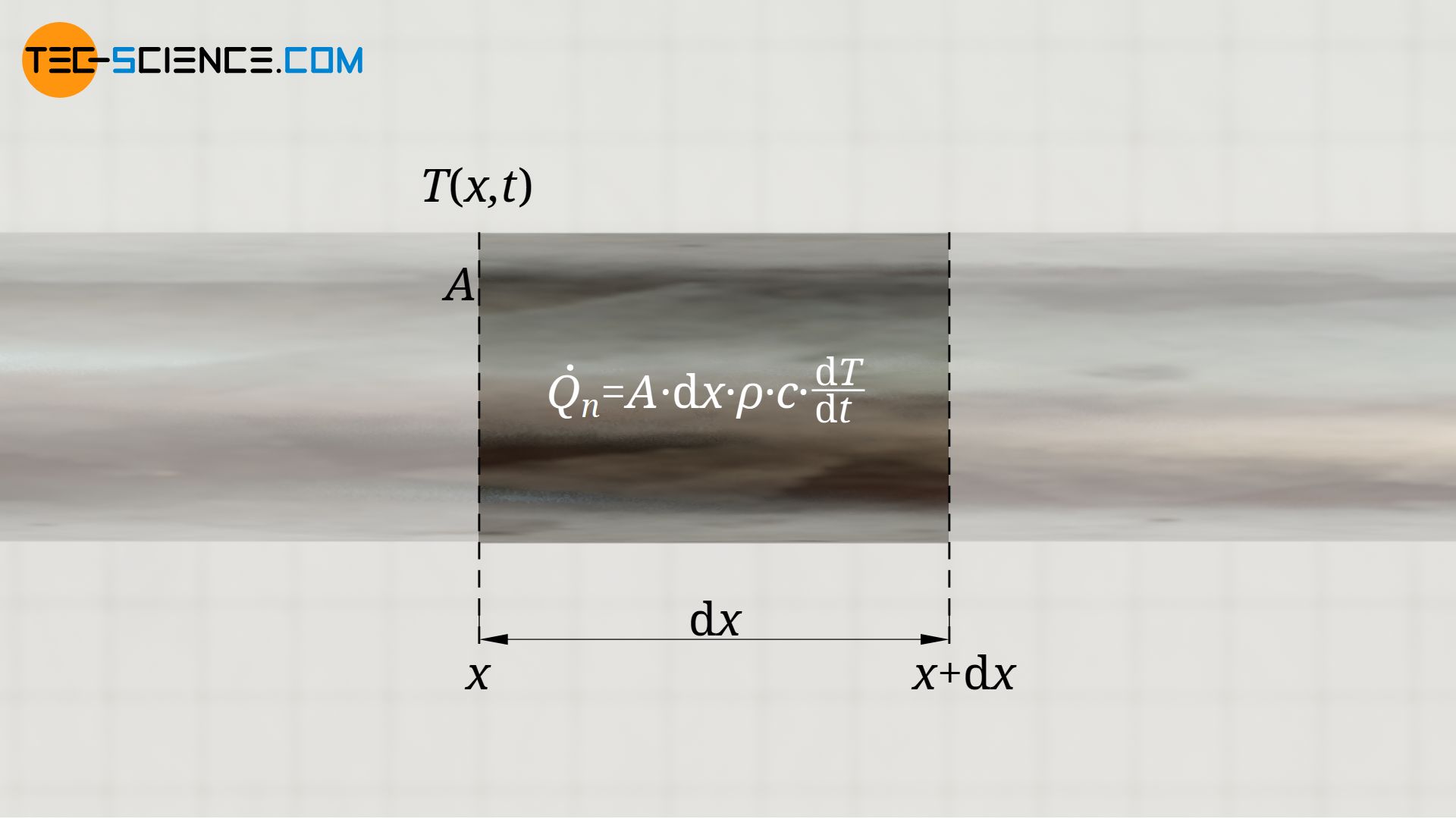
In the above equation, the mass m of the rod section was expressed by its volume V and its density ϱ, whereby the volume in turn can be described by the area A and the length of the section dx.
Since the heat Qn is transferred within the time dt, the following relationship applies between the heat flow rate Q*n=Qn/dt and the temporal change of the temperature dT/dt:
\begin{align}
&\frac{Q_n}{\text{d}t} = A \cdot \text{d}x \cdot \rho \cdot c \cdot \frac{\text{d}T}{\text{d}t} \\[5px]
\label{Q}
&\dot Q_n = A \cdot \text{d}x \cdot \rho \cdot c \cdot \frac{\text{d}T}{\text{d}t} \\[5px]
\end{align}
In the above equation, Q*n denotes the net heat flow that heats or cools the considered section (hence the index “n”). This equation ultimately describes the effect of a heat flow on the temperature, but not the cause of the heat flow itself. The cause of a heat flow is the presence of a temperature gradient dT/dx according to Fourier’s law (λ denotes the thermal conductivity):
\begin{align}
\label{f}
&\underline{\dot Q = – \lambda \cdot A \cdot \frac{\text{d}T}{\text{d}x}} ~~~~~\text{Fourier’s law} \\[5px]
\end{align}
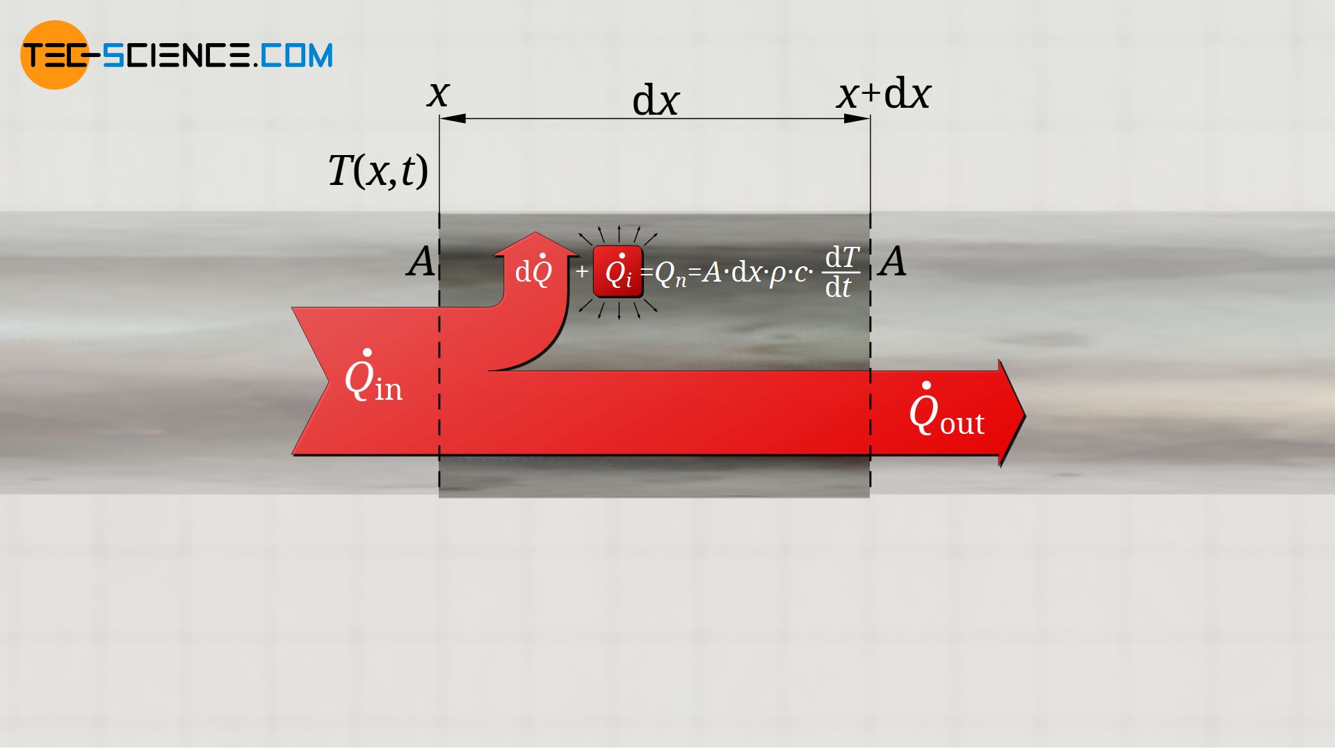
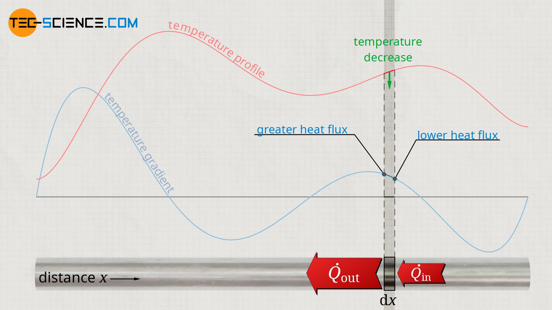
One can determine the net heat flow of the considered section using the Fourier’s law. For this one must determine, on the one hand, which heat flow Q*in leads into the section, and on the other hand, which heat flow Q*out leaves the section. The difference finally corresponds to the net heat flow. The net heat flow is therefore nothing else than the infinitesimal difference dQ* in the heat flows between one end of the section and the other end:
\begin{align}
&\dot Q_n = \dot Q_{\text{out}} – \dot Q_{\text{in}} = {\text{d}\dot Q} \\[5px]
\end{align}
At this point, for a correct mathematical representation it must be noted that an increase in the heat flow along the (positive) x-direction of the rod means that the outgoing heat flow is greater than the incoming heat flow. As a result, heat is removed from the section. This heat must be counted negatively so that the temperature change according to equation (\ref{Q}) actually corresponds to a decrease in temperature (dT<0). Therefore a negative sign must be added to the upper equation:
\begin{align}
&\underline{\dot Q_n =- {\text{d}\dot Q}} \\[5px]
\end{align}
If in equation (\ref{Q}) the net heat flow Q*n is replaced by the difference of the outgoing and incoming heat flow dQ*, then the following relationship applies to the temporal change of the temperature:
\begin{align}
\label{kor}
&-\text{d} \dot Q = A \cdot \text{d}x \cdot \rho \cdot c \cdot \frac{\text{d}T}{\text{d}t} \\[5px]
& \frac{\text{d}T}{\text{d}t} =- \frac{1}{A \cdot \rho \cdot c} \cdot \frac{\text{d} \dot Q}{\text{d}x} \\[5px]
\end{align}
The term dQ*/dx corresponds to the first derivative of the heat flow with respect to x (heat flow gradient). According to Fourier’s law, this in turn corresponds to the second derivative of the temperature with respect to x. The use of the Fourier’s Law (\ref{f}) in the above equation reveals this relationship:
\begin{align}
\require{cancel}
& \frac{\text{d}T}{\text{d}t} =- \frac{1}{A \cdot \rho \cdot c} \cdot \frac{\text{d} \dot Q}{\text{d}x} \\[5px]
& \frac{\text{d}T}{\text{d}t} =- \frac{1}{A \cdot \rho \cdot c} \cdot \frac{\text{d} \left( – \lambda \cdot A \cdot \frac{\text{d}T}{\text{d}x} \right)}{\text{d}x} \\[5px]
& \frac{\text{d}T}{\text{d}t} =- \frac{-\lambda \cdot \bcancel{A}}{\bcancel{A} \cdot \rho \cdot c} \cdot \frac{\text{d} \left(\frac{\text{d}T}{\text{d}x} \right)}{\text{d}x} \\[5px]
& \underline{\frac{\text{d}T}{\text{d}t} = \frac{\lambda}{\rho \cdot c} \cdot \frac{\text{d}^2 T}{\text{d}x^2}} \\[5px]
\end{align}
The temporal change of the temperature at a certain location is therefore given by the second derivative of the temperature distribution (with respect to x). The second derivative corresponds to the change of the temperature gradient at the considered point.
The temporal change of the temperature in a certain point results from the spatial change of the temperature gradient at this point. The heat equation describes for an unsteady state the propagation of the temperature in a material.
In general, temperature is not only a function of time, but also of place, because after all the rod has different temperatures along its length. In the equation above, the left hand side of the equation is therefore a partial derivative of temperature with respect to time and the right hand side of the equation is a second partial derivative with respect to space. The correct mathematical notation is therefore:
\begin{align}
&\boxed{\frac{\partial T(x,t)}{\partial t} = \frac{\lambda}{\rho \cdot c} \cdot \frac{\partial^2 T(x, t)}{\partial x^2}} \\[5px]
\end{align}
This differential equation is a so-called parabolic partial differential equation (second order differential equation).
Explanation and interpretation of the heat equation
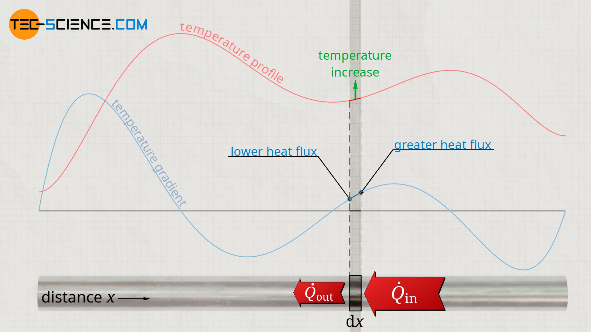
The statement of the heat equation can be clearly illustrated. If the temperature gradient increases at one point (positive change of the temperature gradient ∂²T/∂x²>0), then this means that the temperature gradient is larger at a point just to the right. In this case, much more heat flows into the section under consideration from the right than flows out from the left. Note that the heat flow always flows in the direction of decreasing temperature, in this case from right to left.
In this case, the temperature increases over time in the considered section of the rod. The stronger the change of the temperature gradient, the more the incoming heat flow differs from the outgoing heat flow. This results in a larger net heat flow and thus a temporally stronger increase in temperature.
On the other hand, if the temperature gradient decreases in one point (negative change of the temperature gradient ∂²T/∂x²<0), a smaller temperature gradient is present just to the right of this point. In this case, less heat from the right flows into the considered section, but more heat flows out on the left side. So the temperature decreases in time in the considered section.
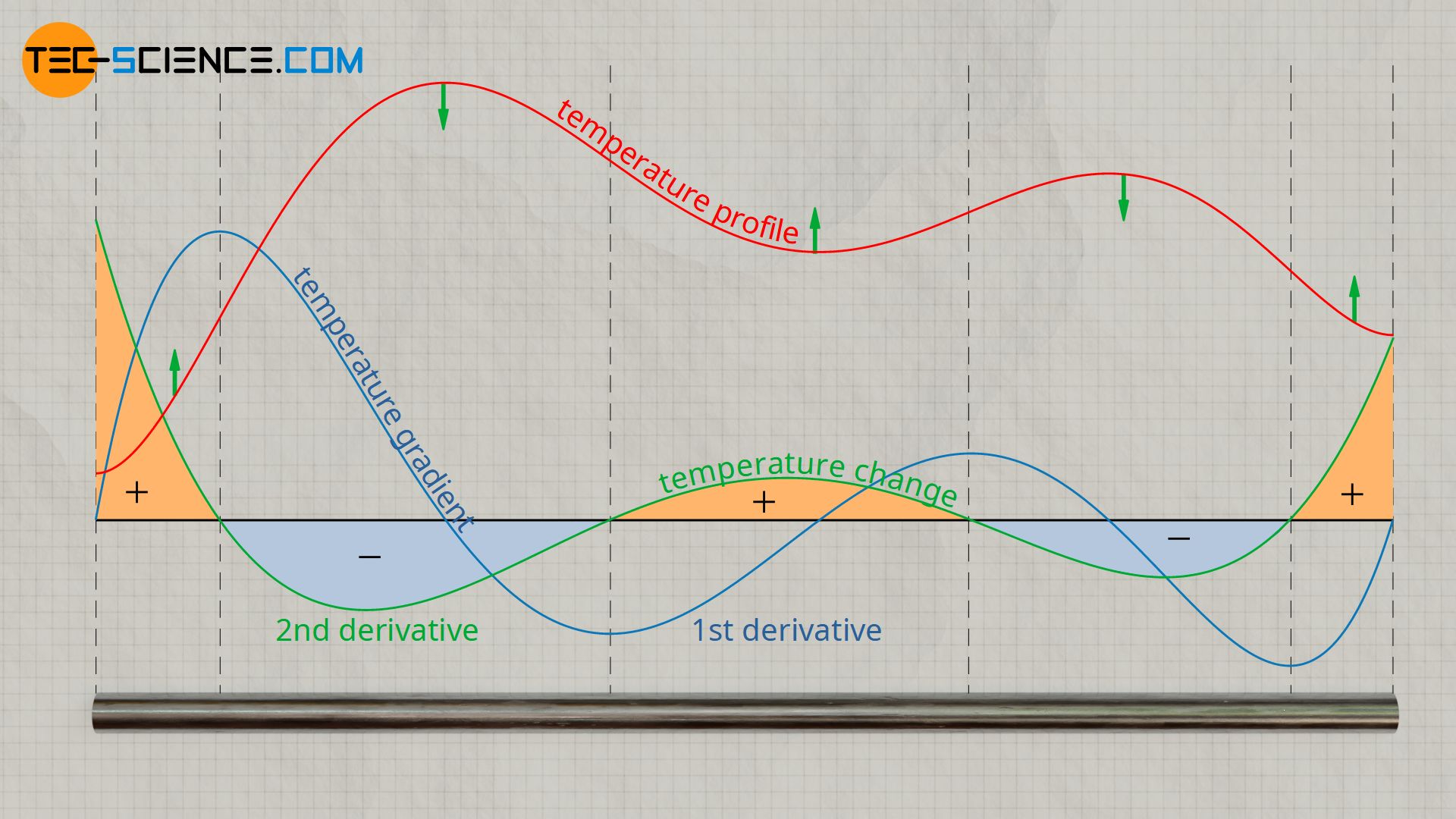
The figure below shows the temperature distribution along the rod at a certain point in time. Furthermore, the temperature gradient is shown as the first derivative of the temperature function with respect to space. The change of this temperature gradient corresponds to the second derivative of the temperature and, according to the heat equation, finally to the temperature change over time. It can be seen from this that in the area of the high points of the temperature distribution the temporal temperature change is negative and in the area of the low points positive. This means that areas with high temperatures cool down and areas with low temperatures heat up. As a result, the temperatures will equalize over time until a constant temperature is finally reached.
Thermal diffusivity
In the following, the solely material-dependent term λ/c⋅ϱ in the heat equation is to be interpreted more closely. This term represents the proportionality constant between the spatial change of temperature gradient and the resulting temporal temperature change. It is obviously true that …
- the greater the thermal conductivity and
- the lower the specific heat capacity and
- the lower the density of the material,
the greater the temporal temperature change.
It becomes clear that thermal conductivity has an influence on temperature change in this way. Because the greater the thermal conductivity, the greater the heat flows entering and leaving a considered section of the material. This results in a large net heat flow, which in turn means a strong change in temperature over time.
The influence of the heat capacity of the material on the temperature change also becomes clear, because the lower the heat capacity, the less heat is required to change the temperature. Therefore, the lower the heat capacity, the greater the temperature change for a given net heat flow.
It also becomes clear very quickly that the change in temperature over time depends on the density of the material. The lower the density, the less mass a section of the rod has. And the lower the mass, the faster a material will heat up or cool down for a given heat flow. Thus it is also clear that a lower density means a greater temperature change.
The term λ/c⋅ϱ thus represents a measure of how quickly the temperature changes with a given change in the temperature gradient. To put it simple, this term indicates how fast the temperature propagates or diffuses in a material. This term is therefore also known as thermal diffusivity “a”:
\begin{align}
& \boxed{\frac{\partial T}{\partial t} = a \cdot \frac{\partial^2 T}{\partial x^2}} ~~~~~\text{mit}~~~ \boxed{a:=\frac{\lambda}{\rho \cdot c}} ~~~~~\text{thermal diffusivity}\\[5px]
\end{align}
Despite the fact that thermal diffusivity and thermal conductivity can be converted into each other, there are still differences in the significance of both quantities. While thermal diffusivity describes the unsteady state of temperature fields, thermal conductivity is used to calculate heat flows in a steady state.
Diffusion equation
The principle statement of the heat equation is that in the presence of different temperatures, heat flows occur, which finally lead to a temperature equalization. The analogous situation is also found with concentration differences in substances. Due to such concentration differences, mass flows occur, which lead to an equalization of the concentrations. It is therefore not surprising that diffusion processes are also described with formally the same equation:
\begin{align}
& \boxed{\frac{\partial u}{\partial t} = k \cdot \frac{\partial^2 u}{\partial x^2}} \\[5px]
\end{align}
The following quantities can be regarded as analogous to one another:
| Quantity | Heat diffusion (thermal conduction) | Mass diffusion |
| u | Temperature | Concentration |
| k | Thermal diffusivity | Mass diffusivity |
So instead of temperature differences, one can simply think of concentration differences (e.g. ink in a glass filled with water). In both cases the equalization process follows the same laws. Conversely, the flow of heat can be regarded as a kind of heat diffusion. For this reason, the heat equation is also called diffusion equation.
Three-dimensional diffusion equation
For a three-dimensional case of heat conduction, heat flows no longer have to be considered in one dimensional direction only, but in all three directions (this also applies to the mass flows in the case of diffusion). In this case, one considers a volume element and balances which heat flows enter the volume element in x-, y- and z-direction and exit on the other side.
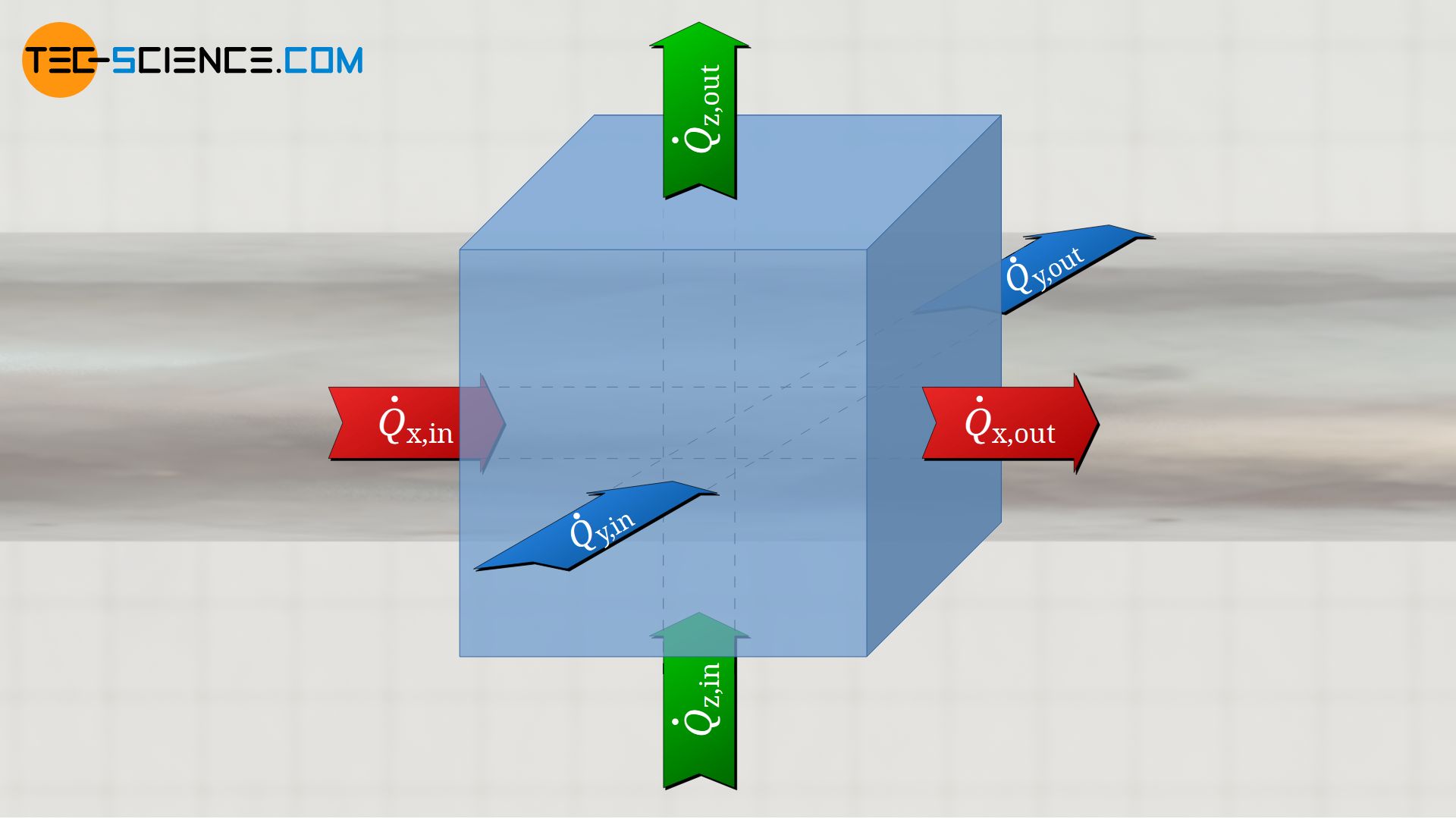
The sum of these individual considerations results in the total net heat flow flowing into or out of the volume element, which then leads to a change in temperature. Thus, the diffusion equation for the three-dimensional case is as follows (assuming isotropic material for which k is identical in all three spatial directions):
\begin{align}
&\boxed{\frac{\partial u(\vec s,t)}{\partial t} = k \cdot \frac{\partial^2 u}{\partial x^2} + k \cdot \frac{\partial^2 u}{\partial y^2} + k \cdot \frac{\partial^2 u}{\partial z^2}} ~~~~~\text{and } ~~ \vec{s} = \left( \begin{array}{c} x \\ y \\ z \\ \end{array}\right) \\[5px]
\end{align}
The sum of the second derivatives is mathematically denoted by the so-called Laplace operator Δ (Note: The Laplace operator must not be confused with the delta sign for differences!):
\begin{align}
&\boxed{\frac{\partial u(\vec s,t)}{\partial t} = k \cdot \Delta u(\vec s, t)} ~~~~~\text{and}~~~\boxed{\Delta = \frac{\partial^2}{\partial x^2} + \frac{\partial^2}{\partial y^2} + \frac{\partial^2}{\partial z^2}} \\[5px]
\end{align}
The simulation below shows the application of the heat equation for a two-dimensional case. The temperature behavior of a plate is simulated, which is heated at two points. The temperature at the edge of the plate was assumed to be constant in time.
Heat equation with internal heat generation
When deriving the heat equation, it was assumed that the net heat flow of a considered section or volume element is only caused by the difference in the heat flows going in and out of the section (due to temperature gradient at the beginning an end of the section). However, chemical reactions inside the material or an internal heat supply can additionally lead to a heat flow. This then also contributes to the temperature change. Taking into account such an internally generated heat flow Q*i, the equation (\ref{kor}) then results as follows:
\begin{align}
&-\text{d}\dot Q + \dot Q_i= A \cdot \text{d}x \cdot \rho \cdot c \cdot \frac{\text{d}T}{\text{d}t} \\[5px]
\end{align}
Rearranging this equation and using Fourier’s law gives the following relationship:
\begin{align}
& \frac{\text{d}T}{\text{d}t} =- \frac{1}{A \cdot \rho \cdot c} \cdot \frac{\text{d}\dot Q}{\text{d}x} + \frac{\dot Q_i}{A \cdot \text{d}x \cdot \rho \cdot c} \\[5px]
& \frac{\text{d}T}{\text{d}t} =\frac{\lambda}{\rho \cdot c} \cdot \frac{\text{d}^2 T}{\text{d}x^2} + \frac{\dot Q_i}{\underbrace{A \cdot \text{d}x }_{dV} \cdot \rho \cdot c } \\[5px]
& \frac{\text{d}T}{\text{d}t} =\frac{\lambda}{\rho \cdot c} \cdot \frac{\text{d}^2 T}{\text{d}x^2} +\frac{1}{\rho \cdot c} \cdot \underbrace{\frac{\dot Q_i}{dV}}_{\dot q_i} \\[5px]
& \frac{\text{d}T}{\text{d}t} =\frac{\lambda}{\rho \cdot c} \cdot \frac{\text{d}^2 T}{\text{d}x^2} +\frac{1}{\rho \cdot c} \cdot \dot q_i \\[5px]
\end{align}
The quantity q*i refers to the internal heat energy generated per unit of time and per unit of volume released at a certain time t at a location x inside the material. For a mathematically correct notation, the one-dimensional heat equation with internal heat generation is thus as follows:
\begin{align}
&\boxed{\frac{\partial T(x,t)}{\partial t} = \frac{\lambda}{\rho \cdot c} \cdot \frac{\partial^2 T(x, t)}{\partial x^2} + \frac{1}{\rho \cdot c} \cdot \dot q_i(x,t) } \\[5px]
\end{align}
The same applies to the three-dimensional case:
\begin{align}
&\boxed{\frac{\partial T(\vec s,t)}{\partial t} = \frac{\lambda}{\rho \cdot c} \cdot \Delta T(\vec s, t) + \frac{1}{\rho \cdot c} \cdot \dot q_i(\vec s,t) } \\[5px]
\end{align}
")


")

