To describe the heat and mass transport, dimensionless numbers are introduced to describe the processes within the boundary layers.
Between a flowing fluid and a solid surface, different boundary layers are formed, which were discussed in detail in the linked articles:
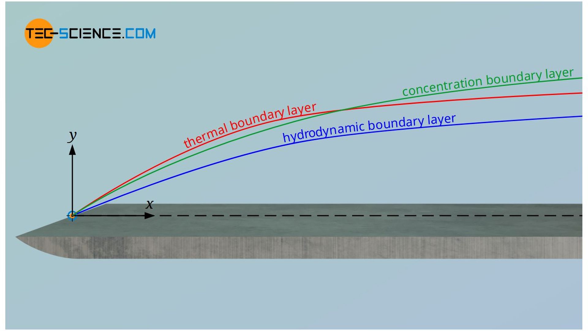
- velocity boundary layer (hydrodynamic boundary layer)
- temperature boundary layer (thermal boundary layer)
- concentration boundary layer (substance boundary layer)
Note that these boundary layers are generally different from each other and do not have the same profile. For example, while a hydrodynamic boundary layer will always develop, a temperature or concentration boundary layer may not always be present. If, for example, the wall and the fluid have the same temperature, then there is no temperature gradient and thus no thermal boundary layer. In a similar way, this applies to the flow of homogeneous fluids that have no concentration gradient and thus no concentration boundary layer.
Characteristic gradients are present in all the boundary layers, which lead to transfer of momentum, heat and mass. The table below compares the respective transport equations. This table has already been discussed in detail in the article Thermal and concentration boundary layer.
| momentum transport | heat transport | mass transport | |
|---|---|---|---|
| law of | Newton | Fourier | Fick |
| \begin{align} \notag &\boxed{\tau = \eta~ \frac{\partial v}{\partial y}} \left(= \dot p_a\right) \end{align} | \begin{align} \notag &\boxed{\dot q = – \lambda ~\frac{\partial T}{\partial y}} \end{align} | \begin{align} \notag &\boxed{\dot n = – D~ \frac{\partial c}{\partial y}} \end{align} | |
| drive | velocity gradient | temperature gradient | concentration gradient |
| characteristic quantity | dynamic viscosity \(\eta\) | thermal conductivity \(\lambda\) | diffusion coefficient \(D\) |
| kinematic Viscosity \begin{align} \notag &\boxed{\nu = \frac{\eta}{\rho}} \\[5px] \end{align} | thermal diffusivity \begin{align} \notag &\boxed{a = \frac{\lambda}{\rho \cdot c_p}} \\[5px] \end{align} | ||
| flux | momentum flux | heat flux | diffusion flux |
Note that the kinematic viscosity ν is directly related to dynamic viscosity by the volumetric mass density. It is therefore also a characteristic quantity of the momentum transport. Likewise, thermal diffusivity “a” is directly related to thermal conductivity by density and specific heat capacity cp and can be regarded as a characteristic quantity for heat transport.
The three boundary layers do not exist independently of each other, but influence each other. For example, a low flow velocity means that heat is not transported very quickly with the flow. This leads to an increased heating of the fluid. This not only changes mass transport by diffusion, but also the temperature-dependent viscosity. This means a changed flow behavior, which in turn influences the heat transport. Thus, the processes in the respective boundary layers influence each other.
So if one wants to compare the momentum, heat and mass transport for systems of different sizes, then this is only possible if the entire boundary layers or the processes taking place within them are in the same ratio. For this reason, a total of three dimensionless similarity parameter are introduced. These dimensionless numbers put two characteristic parameters of the boundary layers in relation to each other. These dimensionless numbers are the Prandtl number Pr, the Schmidt number Sc and the Lewis number Le:
| Prandtl number Pr | Schmidt number Sc | Lewis number Le |
| Ratio of momentum transport to energy transport | ratio of momentum transport to mass transport | ratio of heat transport to mass transport |
| \begin{align} \notag &\boxed{Pr = \frac{\nu}{a}}=\frac{\eta \cdot c_p}{\lambda} \\[5px] \end{align} | \begin{align} \notag &\boxed{Sc = \frac{\nu}{D}} =\frac{\eta}{\rho \cdot D}\\[5px] \end{align} | \begin{align} \notag &\boxed{Le = \frac{a}{D}}=\frac{\lambda}{\rho \cdot c_p \cdot D} \\[5px] \end{align} |
A closer look reveals that the ratio of the Schmidt number to the Prandtl number is the Lewis number:
\begin{align}
\require{cancel}
& \frac{Sc}{Pr}= \frac{\frac{\nu}{D}}{\frac{\nu}{a}}=\frac{\bcancel{\nu} \cdot a}{D \cdot \bcancel{\nu}} = \frac{a}{D }=Le \\[5px]
&\boxed{Le=\frac{Sc}{Pr}}
\end{align}
The three boundary layers are thus completely defined by two dimensionless numbers, since the third number can be determined from them. These dimensionless parameters are of great importance for the transferability of model experiments to reality. Only if these dimensionless parameters are the same for the model as for the real case, can physically similar processes of momentum, heat and mass transport be assumed.
Note that the definitions of the dimensionless numbers are not arbitrary, but are based on the concept of similitude. The dimensionless numbers are therefore also called similarity parameters. These parameters thus offer the possibility of describing flows in a very general way, independent of the size of the system. They are important links between model scale and real scale. Such similarity parameters include, for example, the Reynolds number, which is used to characterize the kinematic flow behavior.
The above-mentioned parameters will be discussed in more detail in the following articles:
")
")


")
