The fatigue test provides information about the strength of a material under continuously changing stress (dynamic load).
Introduction
The intensity of the stress increases slowly but steadily in the tensile, compression and flexural test until the load finally fractures the specimen. Especially for statically loaded components, the strength parameters determined from this tests provide useful values for material selection and component dimensioning.
In most cases, however, components are subject to dynamic loads at which not only the stress intensity changes constantly but also the direction of the stress. Drive shafts, gears, chain links, springs, connecting rods and cylinder head bolts are just a few examples.
Practice shows that components that are subject to constantly changing stress can only withstand lower stress values in the long term than under static stress. Even if the stress always remains below the yield strength of the material, fatigue fracture can still occur over time. In order to examine material samples or entire components under dynamically changing loads (“vibration”), the fatigue test is used.
The strength limits to be met are lower under dynamic load than under static load!
Test setup
The fatigue test not only exposes standardized specimens but also entire components to vibrational loading. For this purpose, the sample is clamped in a device similar to a tensile testing machine. While the lower clamping device is statically connected to the environment, the upper clamping device is dynamically vibrated by resonance. In the simplest case, the specimen is alternately subjected to tensile and compressive stress (alternating stress).
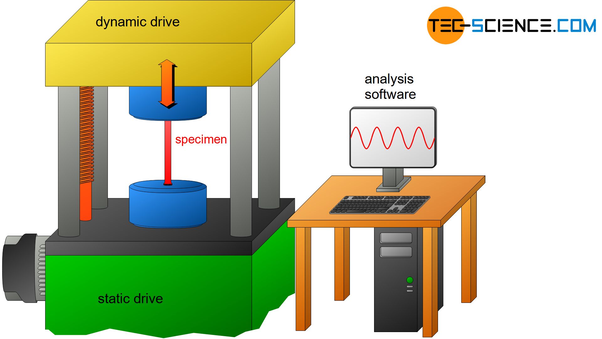
Due to the drive, the oscillations are sinusoidal, some of which have a frequency of more than 200 Hz. Although higher frequencies reduce the testing time, this must not result in an inadmissibly high heating of the specimen.
The static part of the testing machine is equipped with a linear drive. In this way, the table can be lowered or raised in advance of the test.This allows a preload to be applied to the clamped specimen. The stress then oscillates around this previously applied mean stress. Depending on preload, the vibration stress can take place completely in the tensile or in the compression range. In such a case, one no longer speaks of an alternating stress but of a pulsating tensile stress or pulsating compressive stress. Depending on the application, fatigue tests can also be carried out in these load ranges.
Fundamental terms
A complete cycle through the different stress states is called a stress cycle or load cycle. The total number of oscillations (stress cycles) up to a certain point in time is often denoted by the letter \(N\). The number of cycles to failure is represented by \(N_f\) (fatigue life).
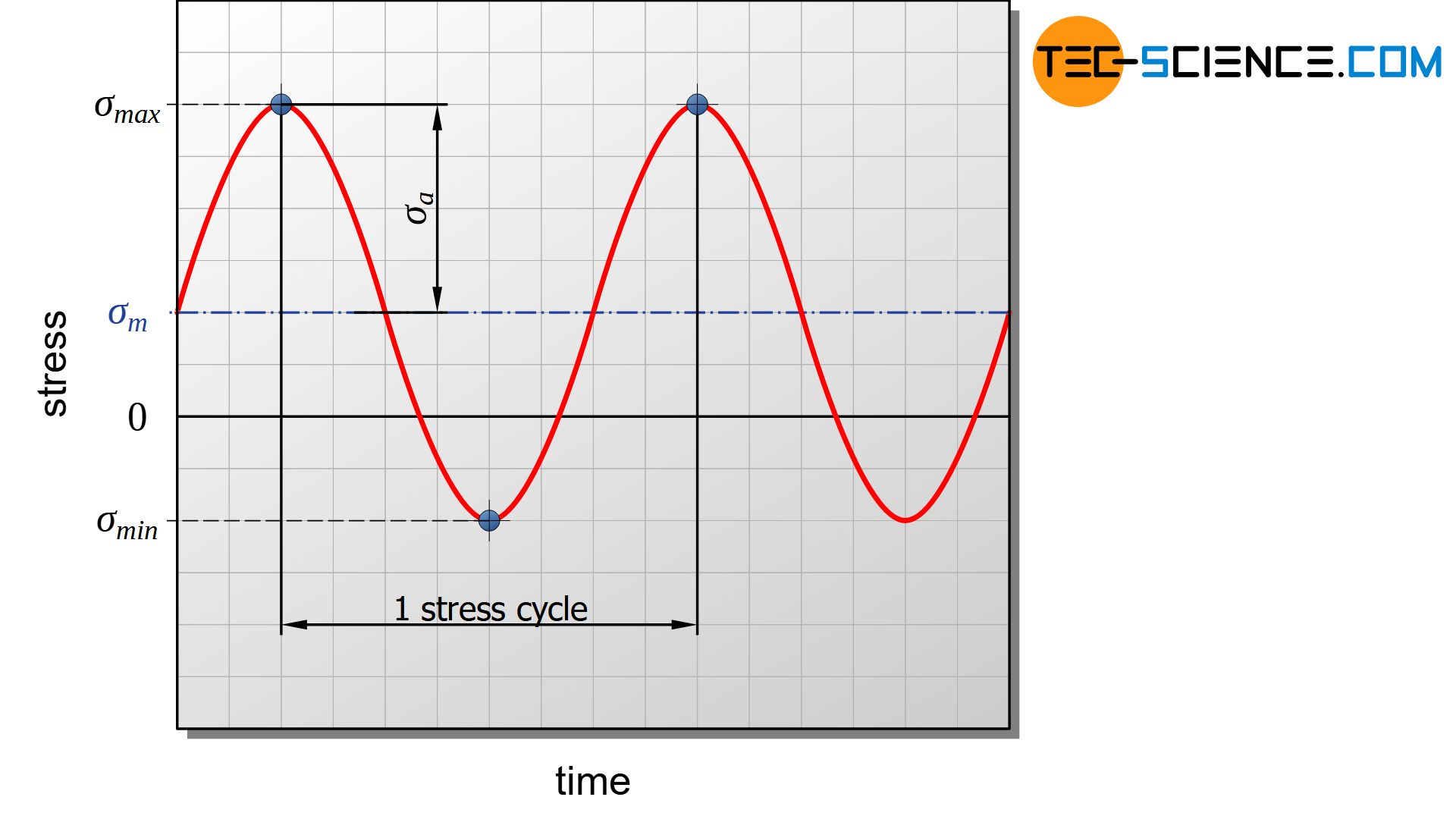
The stress varies during a load cycle between a maximum stress \(\sigma_{max}\) and a minimum stress \(\sigma_{min}\). The mean stress \(\sigma_{m}\) therefore results from the average value of these limit stresses. The stress amplitude is denoted by \(\sigma_a\). The ratio of minimum and maximum stress is called stress ratio \(R\).
\begin{align}
\label{spannungsverhaeltnis}
&\boxed{R = \frac{\sigma_{min}}{\sigma_{max}}} ~~~~~\text{stress ratio} \\[5px]
\end{align}
In the case of alternating stress, the stress ratio is negative, as the maximum stress and the minimum stress differ in sign. A purely alternating stress is present at a stress ratio of \(R\) = -1. Stress ratios greater than zero occur without a change in sign, so that there is a pulsating stress. In the case \(R\) = 0 there is a purely pulsating stress. At a stress ratio of \(R\) = 1, the maximum and minimum stresses are identical, so that this ultimately corresponds to the limit case of static loading.
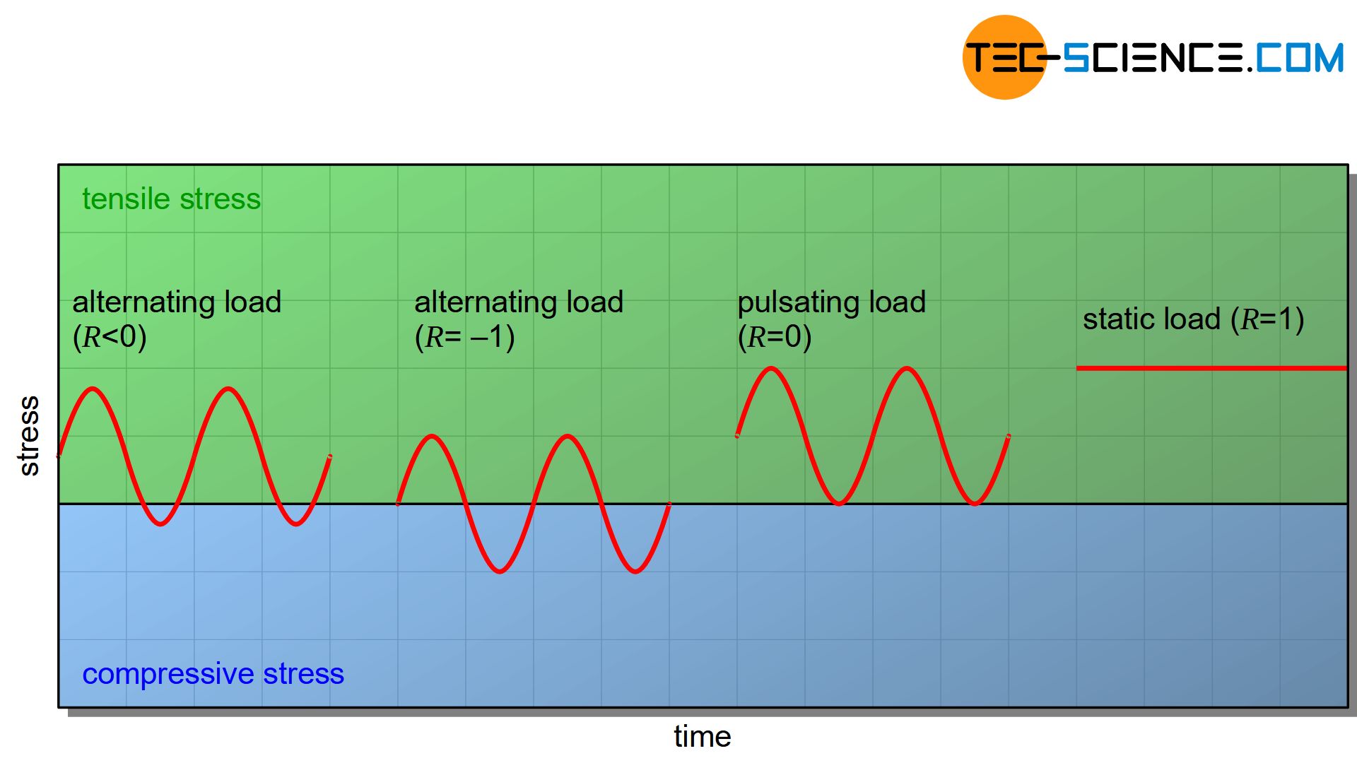
In the case of an alternating stress, not only the stress intensity but also the direction of stress changes. In the case of a pulsating stress, the direction of stress is maintained and only varies in intensity!
Stress-cycle curve (Wöhler curve)
In order to test the fatigue strength of materials, several identical samples of one material are produced in advance. The specimens are then tested one after the other. For each sample, the number of cycles to failure is determined at constant mean stress \(\sigma_m\) and at constant stress amplitude \(\sigma_a\). This procedure is repeated on the other samples. The mean stress is not changed in all tests of a test series. Only the stress amplitude varies from sample to sample. In general, the stress amplitude decreases from sample to sample. Finally, if the stress amplitude is sufficiently small, there will be no more rupture. The sample is therefore considered to be fatigue-resistant.
In the fatigue test, several identical samples are dynamically loaded with different stress amplitudes and the respective number of cycles to failure is determined!
If for each tested sample the respective stress amplitude \(\sigma_a\) is plotted against the number of endured cycles \(N_f\), the so-called stress-cycle curve is obtained. Due to the extreme range of load cycles, a logarithmic scale is chosen on the horizontal axis.
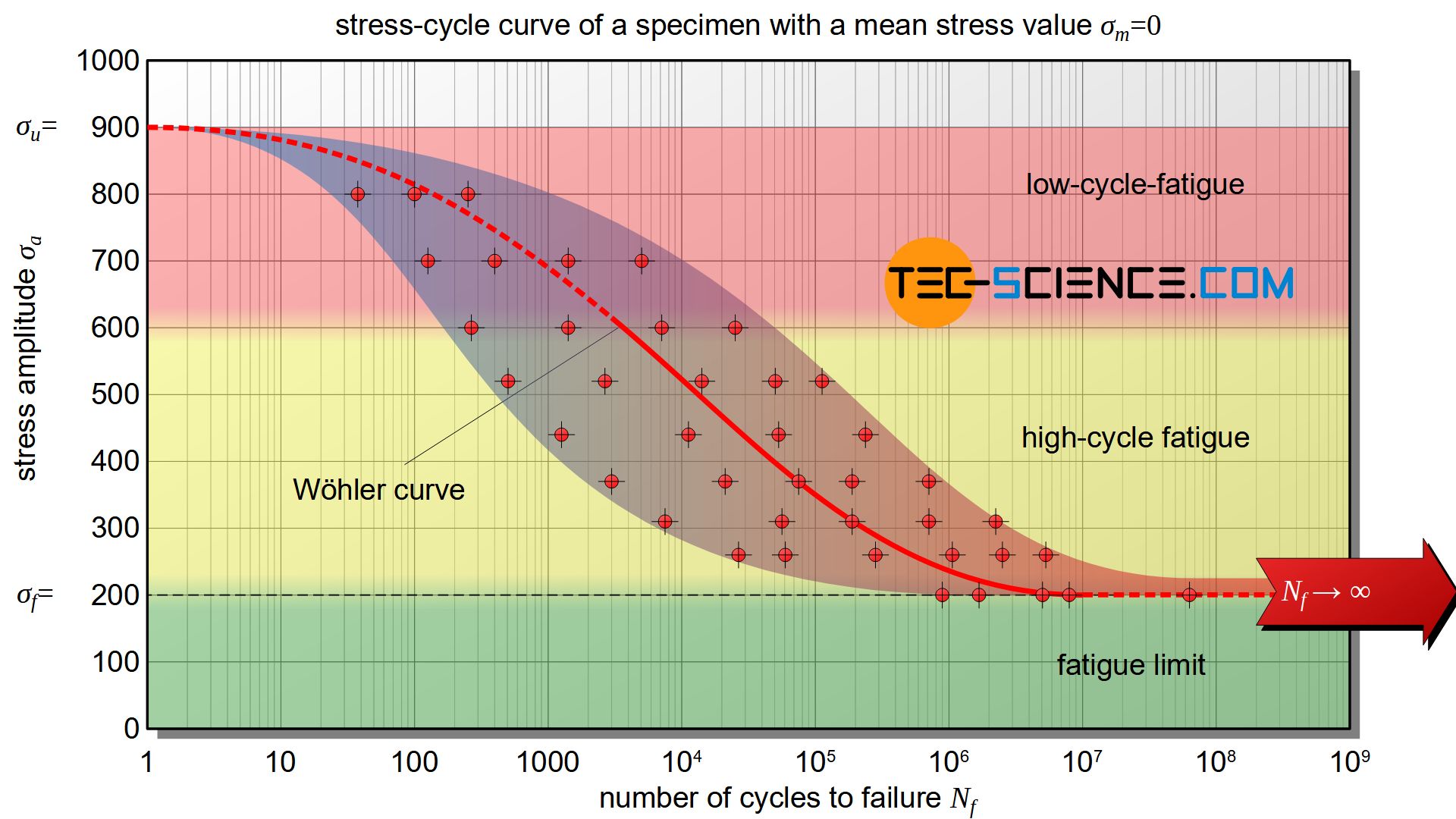
The obtained curve in the diagram is often called Wöhler curve. The Wöhler curve results after a statistical evaluation of several samples, which were tested with identical stress amplitude. Such a statistical evaluation is necessary because the number of load cycles to failure scatters very strong, even with identical stress amplitudes. The high scatter is a result of production-related differences in the microstructure during sample preparation. Such differences can never be completely avoided. Even minor surface impurities can lead to premature cracking and premature breakage of the sample. In this respect, the Wöhler curve is to be interpreted as a probability curve in which, for example, 50 % of the samples reach the respective number of load cycles.
The Wöhler curve is to be interpreted as a probability curve that indicates the number of load cycles after which a sample is expected to break at a given stress amplitude. Wöhler curves are only valid for a certain mean stress!
Note: The Wöhler curve is only used for the evaluation of fatigue tests. Such a diagram is not very informative for the engineer, as the Wöhler diagram is limited to one mean stress only. Therefore, special fatigue limit diagrams are created. The Haigh diagram (goodman diagram) and the Smith diagram are of particular importance. More information can be found in the article Fatigue limit diagram according to Haigh and Smith.
Strength areas
In principle, three areas can be distinguished in the stress-cycle diagram. At high amplitudes, the sample already fractures after relatively few load cycles. This characterizes the area of the so-called low-cycle fatigue. In this area, a sample can only withstand a maximum of 10,000 to 100,000 stress cycles until it breaks. This area is of little importance in practice and is therefore almost not tested, as significantly higher load cycles are required for most applications.
More stress cycles are only possible if the stress amplitude is reduced accordingly. The diagram shows this in the rapidly falling Wöhler curve. This decrease indicates the area of high-cycle fatigue. The transition from low-cycle fatigue to high-cycle fatigue is always smooth and is not subject to any fixed definition.
Higher numbers of load cycles can only be achieved with significantly reduced stress amplitude. Finally, there is no fracture below a certain stress amplitude. Accordingly, the Wöhler curve changes into a horizontal line. This indicates the area of fatigue strength or fatigue limit (more on the differences see section fatigue limit and fatigue strength). This fatigue limit is achieved for ferritic steels from about 1 million to 10 million stress cycles. Samples that pass the fatigue test without fracture up to this number of load cycles are referred to as run-throughs and are considered to be fatigue-resistant.
Note: If the stress amplitude at a pure tensile-compressive alternating loading corresponds to the tensile strength of the sample, the sample will break within the first load cycle. Therefore, in this case the Wöhler curve for decreasing numbers of load cycles approaches the value of the tensile strength more and more.
In the rarely tested area of low-cycle fatigue, samples already fracture after a few load cycles (<100,000). In the area of high-cycle fatigue, the number of load cycles is up to 10,000,000. Beyond this number of load cycles, the samples are considered to be fatigue-resistant.
Influence of mean stress on the Wöhler curve
The mean stress has a particular influence on the course of the Wöhler curve. With the same stress amplitude, a higher mean stress (\(\sigma_m>0\)) causes a higher maximum and minimum stress. As a result, the sample is subjected to greater loads. In spite of the same stress amplitude, the sample breaks at lower load cycles. Consequently, the same number of stress cycles with a higher mean stress can only be achieved by a reduction in the stress amplitude. The Wöhler curve for mean stresses greater zero (\(\sigma_m>0\)) is therefore shifted downwards compared to zero mean stress.
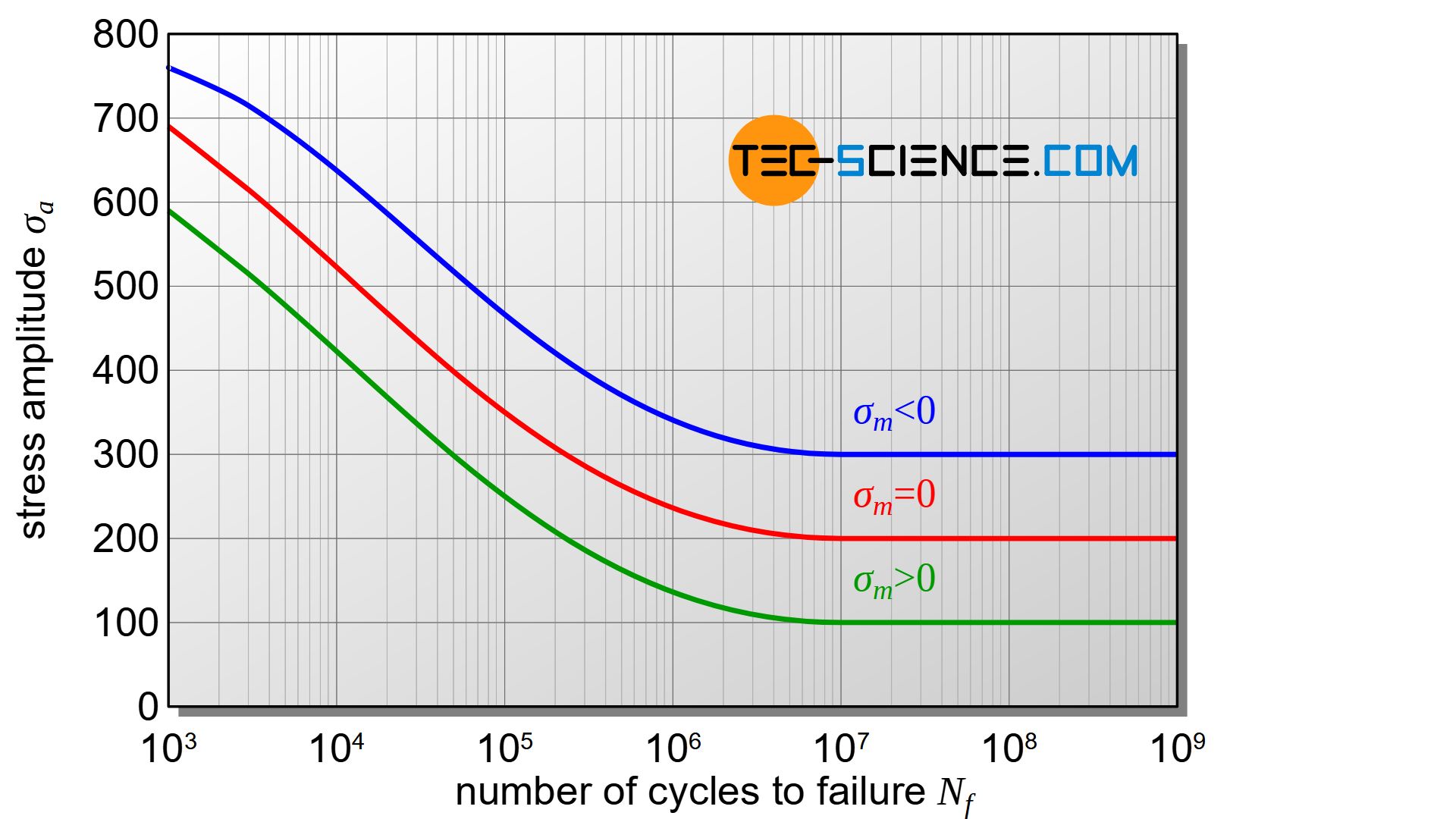
If, on the other hand, the mean stresses are shifted into the negative compression range (\(\sigma_m<0\)) , the opposite effect becomes apparent within certain limits. Despite the same stress amplitude, the sample can then endure a higher number of load cycles. This means that at a given number of stress cycles the stress amplitude can therefore be increased. The Wöhler curve is shifted upwards compared to zero mean stress.
The reason for the increased fatigue resistance at compressive mean stresses is due to the fracture mechanism. Fatigue fracture is usually caused by microcracks in the specimen surface. These microcracks crack more and more under tensile stress. Thus the crack spreads more and more into the interior of the material with each load cycle. With a compressive load, on the other hand, the cracks “close” and crack formation or crack growth is made more difficult (more on this in the section on fracture mechanism).
With greater (tensile) mean stresses, the Wöhler curve is shifted towards lower stress amplitudes!
Thus, in many cases compressive stresses have a more favourable effect on the fatigue strength than tensile stresses. The introduction of residual compressive stresses by shot peening is also based on this principle (more on this in the section Influencing the fatigue strength).
Fatigue limit and fatigue strength
In the case of body centered cubic materials (bcc), a pronounced fatigue-resistance can often be determined (horizontal line in the Wöhler diagram). On the other hand, with face centered cubic materials (fcc), there is usually no fatigue-resistance in the literal sense of the word. For these materials, the Wöhler curve drops over the entire load cycle range. Corrosive media can also cause such behaviour.
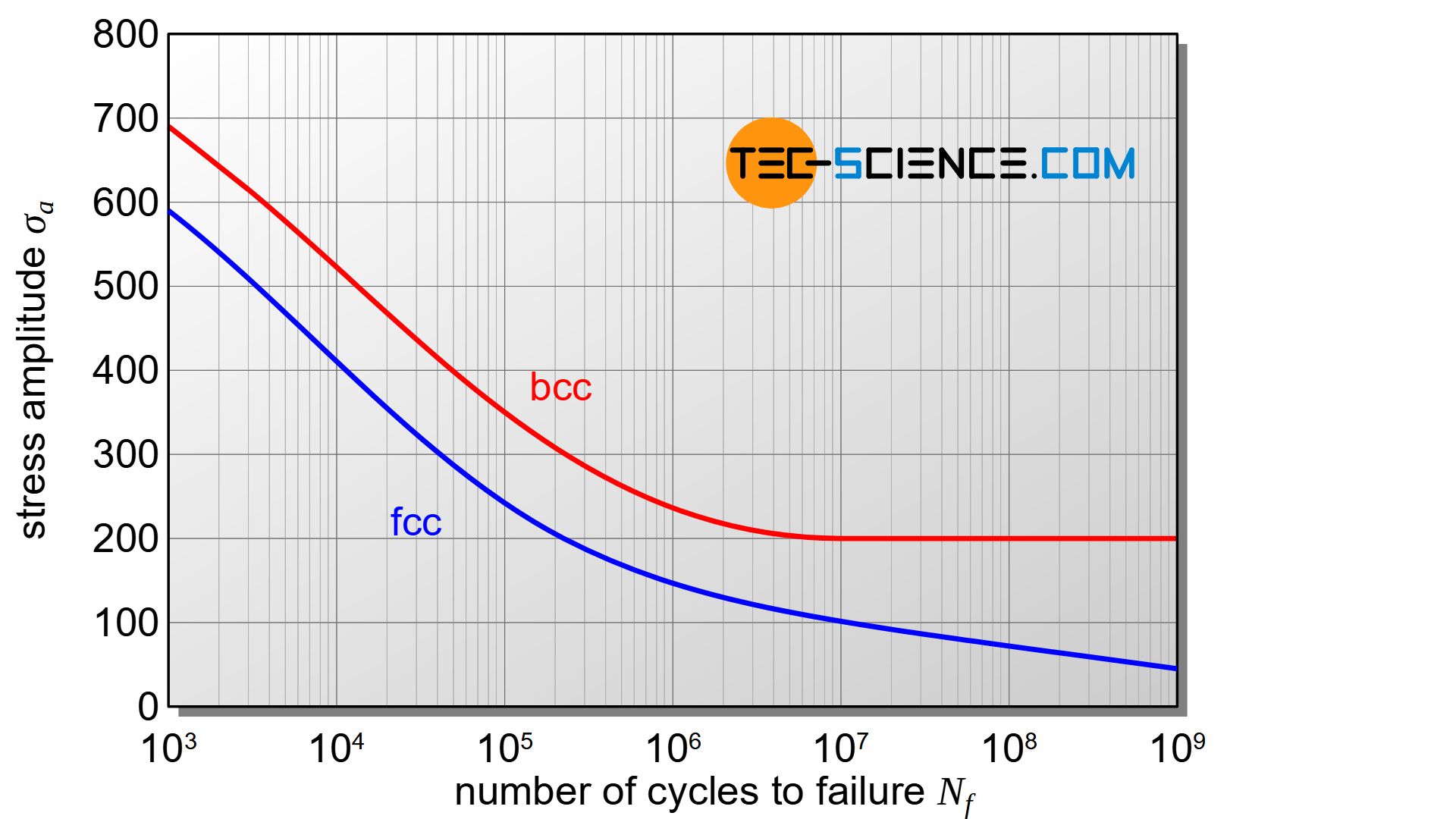
This means that even at the smallest stress amplitudes, the sample will eventually break under a sufficiently large number of load cycles. However, since in practice more than 100 million load cycles rarely occur, samples that can withstand this number without fracture are also referred to as “fatigue-resistant“.
Fatigue limit
The stress amplitude that a sample can withstand without breaking is called fatigue limit \(\sigma_f\) (also referred to as endurance limit). The indication of fatigue limit includes the mean stress \(\sigma_m\) and the stress amplitude \(\sigma_a\):
\begin{align}
\label{dauerschwingfestigkeit}
&\boxed{\sigma_f = \sigma_m \pm \sigma_a} ~~~~~\text{indication of fatigue limit } \\[5px]
\end{align}
Fatigue limit (endurance limit) is defined as the stress amplitude that a sample can withstand permanently or for a sufficiently long number of load cycles at a given mean stress without breaking!
Important special cases arise in the case of a purely alternating load (\(R=-1\)) and a purely pulsating load (\(R=0\)). In the case of pure alternating stress with \(\sigma_m=0\), the fatigue limit is then referred to as alternating fatigue limit \(\sigma_{fa}\) and for pure pulsating stress with \(\sigma_m=\sigma_a\) as pulsating fatigue limit \(\sigma_{fp}\).
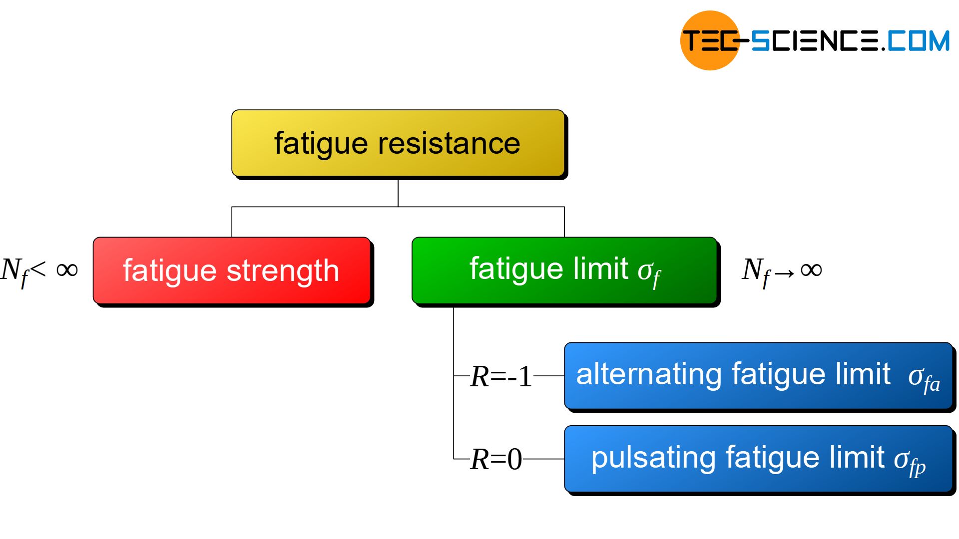
Alternating fatigue limit and pulsating fatigue limit are special cases for fatigue limits for a purely alternating load (mean stress = 0) or a purely pulsating load (mean stress = stress amplitude)!
Fatigue strength
Even if components are subjected to dynamic stress, they do not always have to be designed for fatigue limit for economic reasons. In general, components are not subjected to an infinite number of stress cycles, but only within their intended service life. Percussion drills, for example, are not designed to survive countless years without damage. This means that components are generally only assigned a certain number of load cycles, which they must withstand without damage. This “service strength” is then not called fatigue limit but fatigue strength.
Fatigue strength is defined as the stress amplitude that a material can withstand at a given mean stress for a certain number of load cycles without breaking!
Note that the distinction in the terms fatigue strength and fatigue limit (or fatigue endurance) is often not made in practice and therefore these terms are often used synonymously!
Fracture mechanism
In order to influence the fatigue strength of components, it is necessary to understand the mechanisms underlying the development of fatigue fracture.
Stages of crack formation
The initial cause of fatigue is cracks or other surface defects in the specimen surface. Microscopically, no material surface is perfectly smooth and flat but has roughness and the finest cracks or other inclusions. Such roughnesses act like small notches on which increased stresses with a triaxial stress state arise. These stresses can then be far higher than the uniaxial nominal stresses.
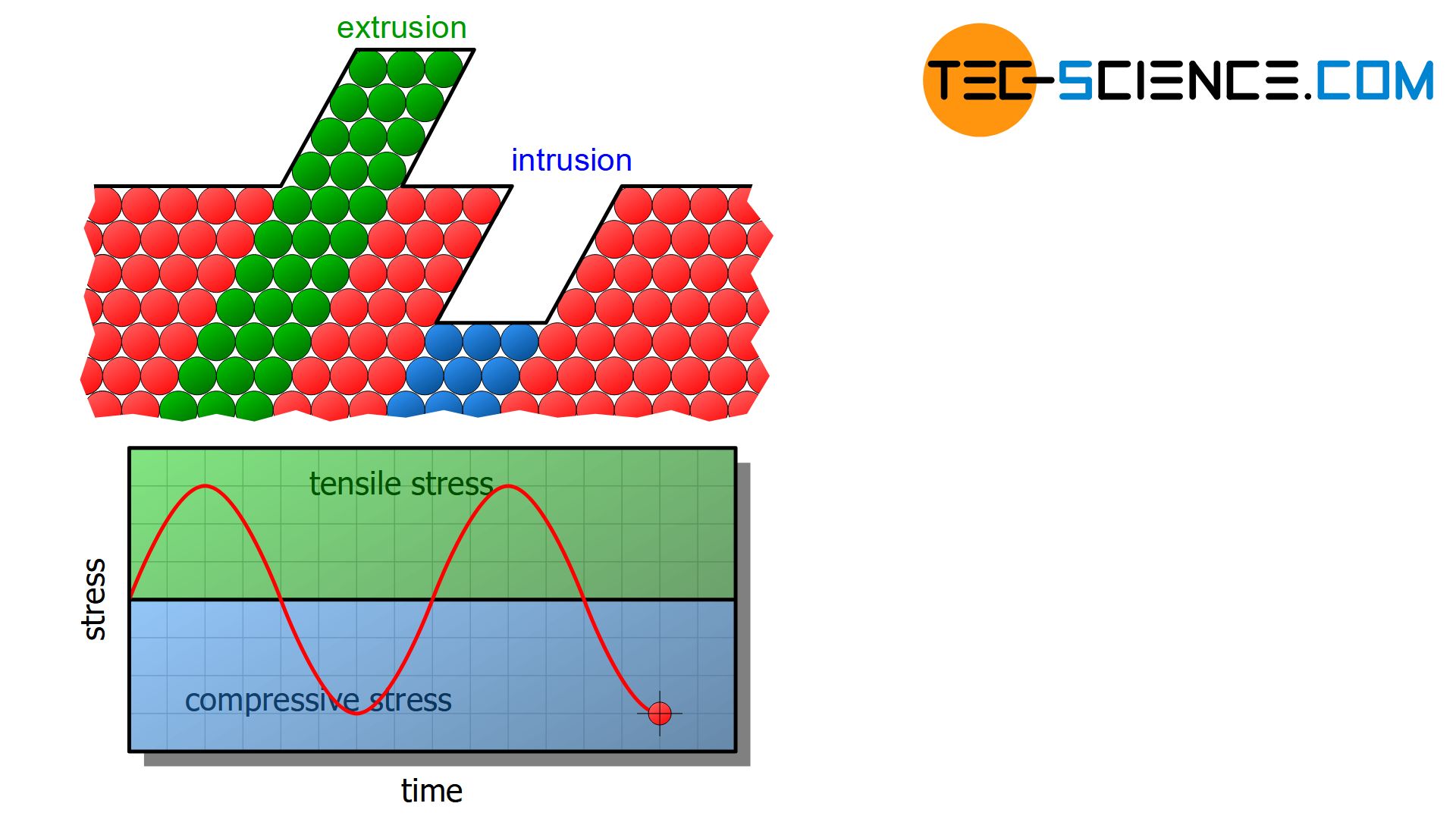
The yield point is then locally exceeded at these flaws and microplastic deformations occur. Material shifts are caused by run-out slip planes. Such shifts leave either bulges (extrusions) or indentations (intrusions) on the surface. These microscopic distortions in turn serve as notches and thus intensify the formation of cracks (stage I).
As a result of the microscopic deformation, hardening effects and thus dislocation build-up can occur. As a consequence, the material will locally embrittle at these points. The material breaks more and more open during a load change and the crack progresses deeper into the interior. This crack propagation marks the onset of fatigue fracture (stage II). However, until the final fracture occurs, countless load changes will usually still take place.
As the crack propagation progresses, the load-bearing residual cross-section decreases more and more. In this way, the load is distributed over an ever smaller area. Sooner or later, the decreasing cross-section will no longer be able to withstand the stress. The tensile strength is exceeded in the remaining cross section and the component finally fractures (stage III). Depending on the material, the fracture surface in this area shows the typical characteristic of a brittle or ductile forced fracture as known from the tensile test.
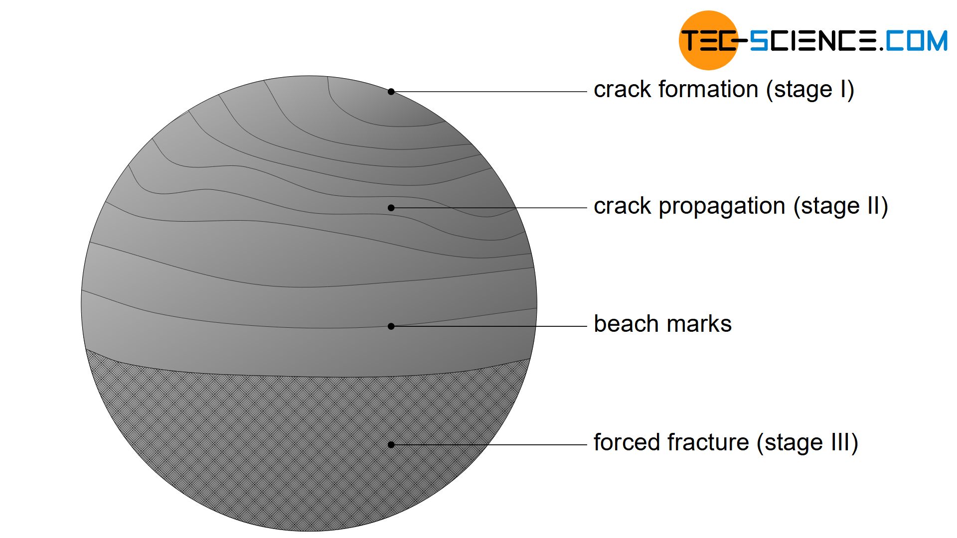
Increased stresses at imperfections lead to local exceeding of the yield strength and thus to the formation of an incipient crack (stage I). The crack spreads more and more with every load change (stage II), until the reduction of the load-bearing cross-section finally leads to a forced fracture (stage III)!
Fatigue striations and beach marks
Due to the cyclic progress of the crack with each load change, typical fatigue striations occur in the material during crack propagation (stage II). These fine structures can only be resolved with the aid of scanning electron microscopes or scanning tunneling microscopes.
However, whenever a strong change occurs in the intensity of stress, the fatigue striations can appear as so-called beach marks. These marks become visible to the naked eye (see figure above). The aforementioned stress changes include not only the rest phases but also strong load changes, which can be directional as well as intensity-related. Such a multi-stage load usually exists in reality, since many components such as the drive shafts of automobiles, are usually never subjected to uniform dynamic stress.
Beach marks become visible because a change in stress intensity is always associated with a change in the velocity of crack propagation. This in turn has an effect on the oxidation of the crack front. Such differently oxidized crack fronts can then be seen with the naked eye.
Beach marks are visible lines on the fracture surface that occur during crack propagation due to oxidation processes!
Since the beach marks are always perpendicular to the direction of crack propagation, the initial point of the crack can also be determined relatively easily. Are the time intervals of the load changes known, which each leave a certain line, the number of beach marks can be used to determine the time at which the crack starts to spread (similar to the annual rings of a tree).
Fatigue fracture surface
A fatigue fracture can therefore be detected by its two typical fracture areas. In the area of crack propagation, the characteristic beach marks or at least fatigue striations are visible. This striation surface is usually relatively smooth due to the permanent microscopic friction of the two fracture halves. In contrast, the forced fracture surface (residual fracture surface) has a rather ragged surface structure.
A fatigue fracture is usually marked by two delimitable areas based on the fracture surface: Area of crack propagation with visible beach marks and the area of forced fracture!
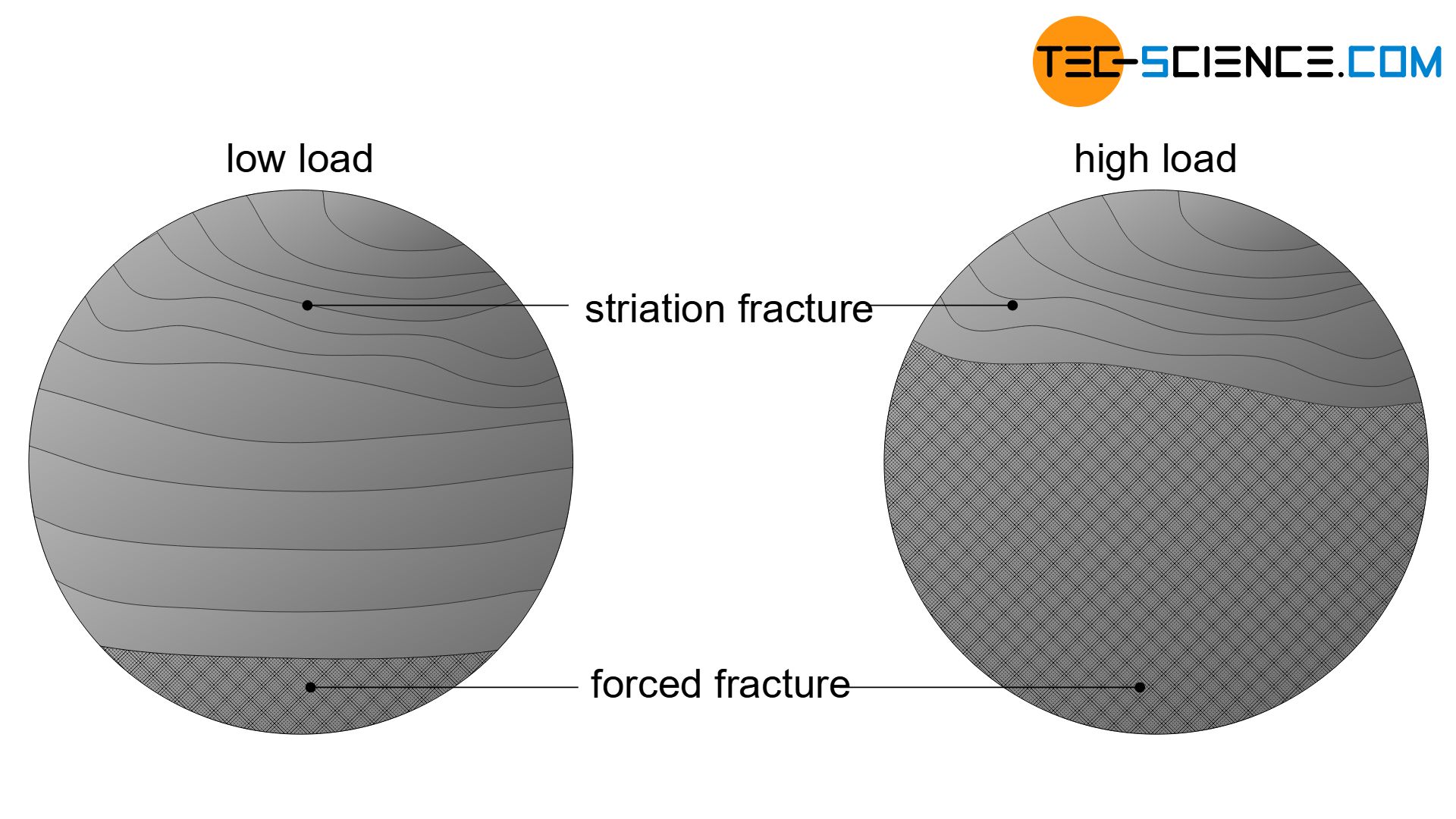
The ratio of the striation fracture surface and the forced fracture surface can also be used to determine the level of the dynamic load. Relatively large areas of forced fracture indicate a high load, while relatively small areas of forced fracture indicate a rather low load.
Note: In general, no beach marks can be found on the broken samples in the fatigue test, as this is not a multi-stage load but a single-stage load with constant stress amplitude (uniform dynamic load).
Influencing the fatigue strength
As explained in the section on fracture mechanisms, flaws on the surface of components usually form the starting point for crack formation. Microcracks on the surface of rough specimens or sharp edges (e.g. in drill holes) act like notches at which very high stress peaks occur. This also applies to corroded areas. All these surface areas favour the formation of cracks and premature breaking of the component.
Thus, the quality of the sample surface obviously has a special influence on the number of cycles to failure. Polished specimens with soft geometry transitions generally have higher fatigue strength values. Therefore, notches, edges and sharp transitions within the components should be avoided.
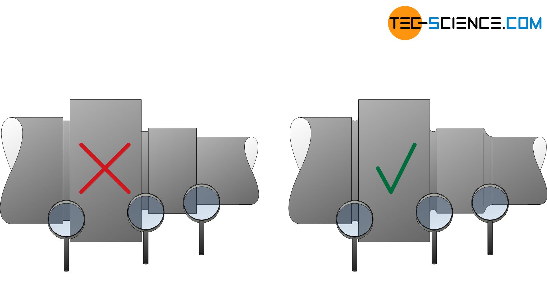
Sharp geometry transitions on components should be avoided to avoid stress peaks in order to increase fatigue strength!
Influence of residual compressive stresses
The dynamic preloading of the specimen also influences the fatigue strength. If a sample is dynamically pre-stressed in advance with a relatively low stress amplitude, this can have a positive effect on the fatigue strength. Such a pre-loaded specimen may withstand a higher number of load cycles in a subsequent fatigue test than a novel specimen.
This may seem paradoxical at first, but is due to the hardening effect of the surface and the resulting residual compressive stresses. Under compressive stresses, crack formation or crack propagation is inhibited, since the compressive forces try to close a possible crack and not to tear it open further.
Preloading of components can have a positive effect on fatigue strength due to hardening effects!
Residual compressive stresses can be introduced by strain hardening, surface hardening or shot peening, for example. In shot peening, fine particles are shot at high speed onto the component surface. In this way, plastic deformations occur on the surface, which then lead to residual compressive stresses in the surrounding elastic areas. Shot peening is very often used, for example, for springs.
Surface hardening in the form of nitriding is also particularly important for increasing the fatigue strength by introducing residual compressive stresses. The alloying elements that combine to form nitrides on the surface of the component generate high residual compressive stresses due to their increased volume.
The introduction of residual compressive stresses (e.g. by shot peening or nitriding) can increase the fatigue strength of components!
Influence of sample size
Not only the surface of the sample but also the sample size itself influences the fatigue strength. For example, larger samples have statistically more “impurities” than smaller samples. For identical materials, therefore, larger samples generally show lower fatigue strength values than smaller specimens with geometrically similar dimensions. This phenomenon is particularly evident with bending and torsional loads, which cause a linear stress curve in the component and thus produce the greatest stress values in the region of the surface.
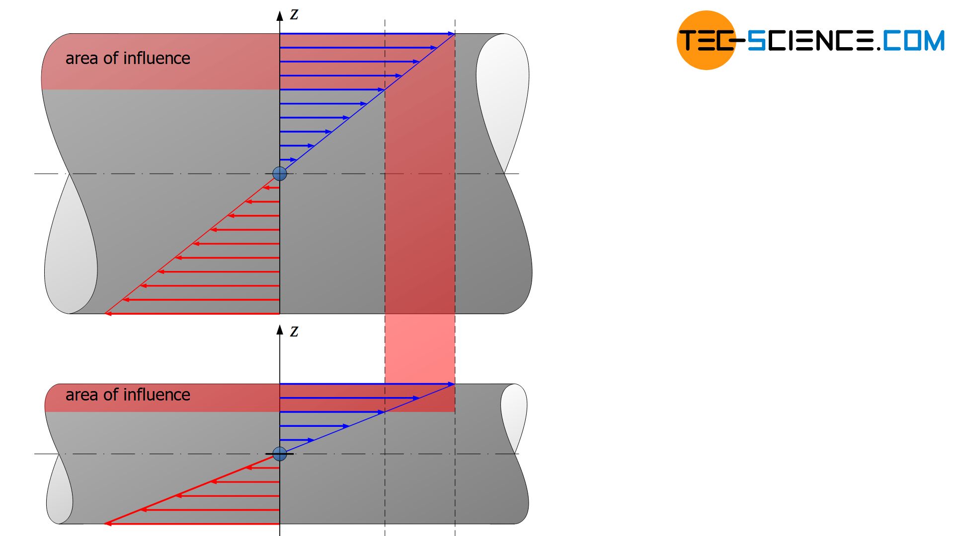
The figure above shows the stress distribution of two specimens subjected to bending load. With identical maximum bending stresses, the same stress range for the larger specimen also covers a larger area. The (enlarged or reduced) region near the surface is therefore of particular importance in these load cases and the influence of the component size is correspondingly large. For dynamic tensile and compressive loads, however, the influence of size is rather less pronounced.
Large components usually have lower fatigue strength values than smaller components!
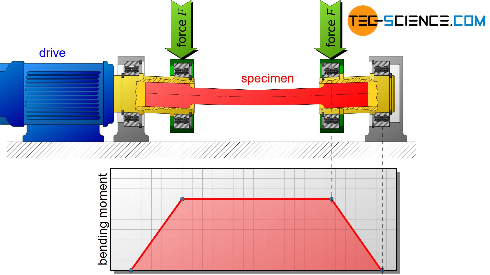
Rotating bending test and reverse bend test
A special type of fatigue test is the rotating bending test, where a round specimen is subjected to an alternating bending stress in order to test bending fatigue strength. Due to the constant bending moment and rotation, the tensile and compressive stresses produced in the material change permanently. During one revolution, each area of the shaft is subjected to tension once and compression half a turn later. In a similar way, the reverse bend test for flat specimens was developed (“back and forth bending test”).


")
")
")