The tensile test is used to determine the strength (yield point, ultimate tensile strength) and toughness (elongation at break) of a material!
Setup
The tensile test is one of the most important testing methods for characterizing or obtaining material parameters. In the tensile test, for example, it is determined which load a material can withstand until it begins to deform plastically (yield strength) or under which maximum load the material breaks (tensile strength). The tensile test can also be used to determine the elongation at break (fracture strain) in order to obtain information about the toughness of a material.
Although the tensile test examines the material behaviour under a pure tensile load, conclusions can also be drawn about the behaviour under other types of load. The tensile test therefore plays a central role in mechanical engineering.
The tensile test is one of the most important tests for determining material parameters in mechanical engineering!
In the tensile test, a material sample with standardized geometry (tensile test specimen) is subjected to a tensile load. Standardization of the geometry is intended to achieve comparability of the material parameters obtained, since the characteristic values are also dependent on the specimen geometry.
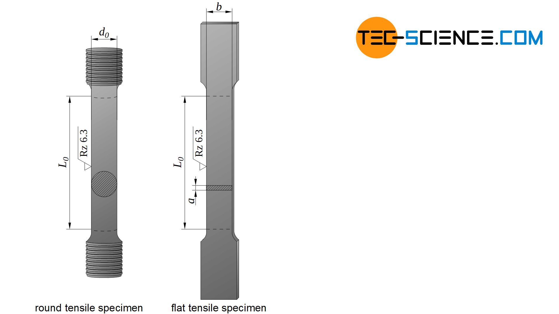
Generally tensile specimens with circular cross-sections are used. These are round bars whose gage length is in a certain ratio to the diameter. While in the USA mainly specimens with four times the length compared to the diameter are used, in Germany lengths with ten times the diameter are often used.
\begin{align}
\label{proportionalstab}
&L_0 = 4 \cdot d_0 &&\text{USA} \\[5px]
&L_0 = 10 \cdot d_0 &&\text{Germany} \\[5px]
\end{align}
In addition to such round tensile specimens, flat tensile specimens with a rectangular cross-section are also used in some cases. Flat tensile specimens are mainly used for testing sheet metal materials. Other geometries are also possible in special cases.
The tensile specimen is now subjected to a quasi-static load in the tensile test under increasing (uniaxial) tensile loading until the sample fractures. For this purpose the tensile test specimen is clamped in the universal testing machine and then the elongation ∆L is measured as a function of the tensile force F.
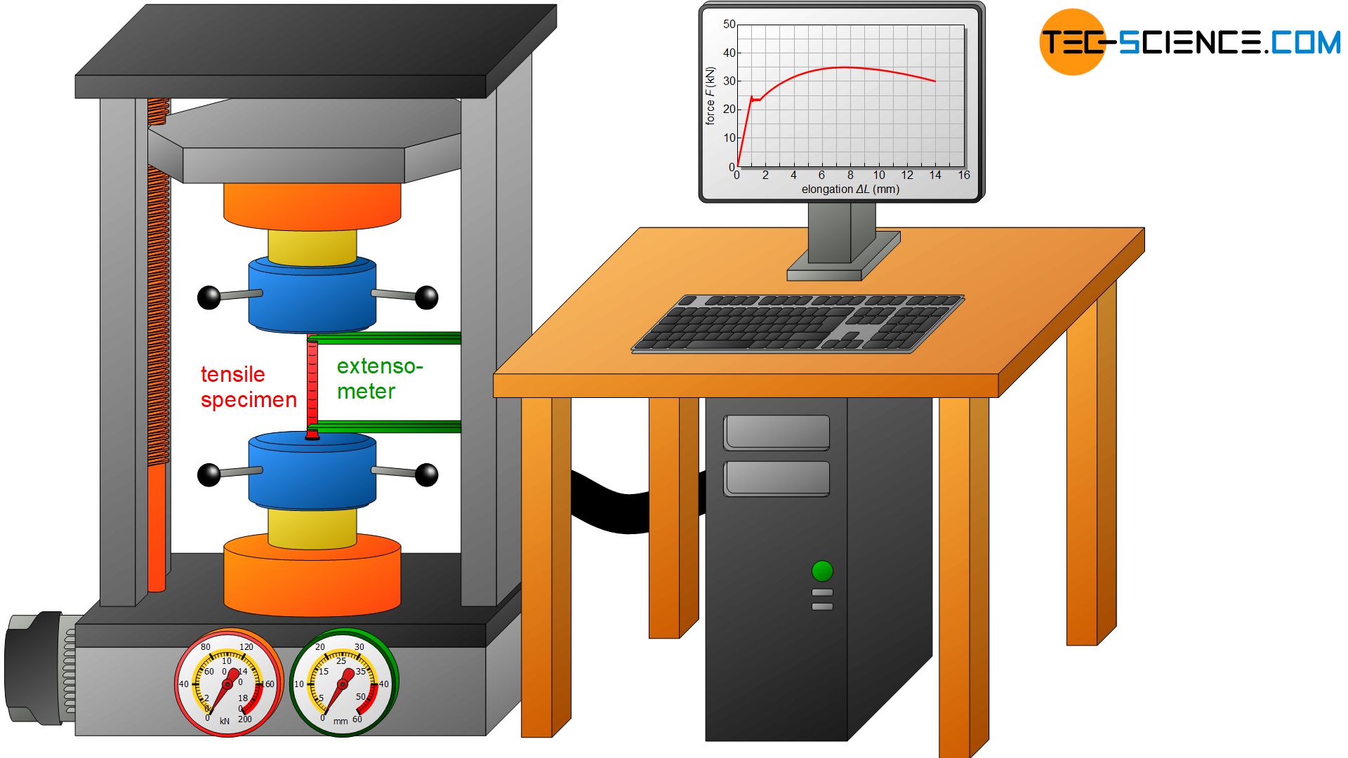
In the tensile test, a standardized specimen is loaded under uniaxial tensile force until it breaks. The force is recorded as a function of the elongation!
In order not to distort the result, the deformation speeds and other details are specified in the corresponding standards. For example, high deformation speeds could lead to an unacceptable heating of the sample and thus also falsify the result. For steels, for example, the increase in stress must not exceed 30 N/mm² per second.
Force-elongation curve
The result of a tensile test is always a force-elongation-curve showing the specimen elongation on the horizontal axis and the applied force on the vertical axis.
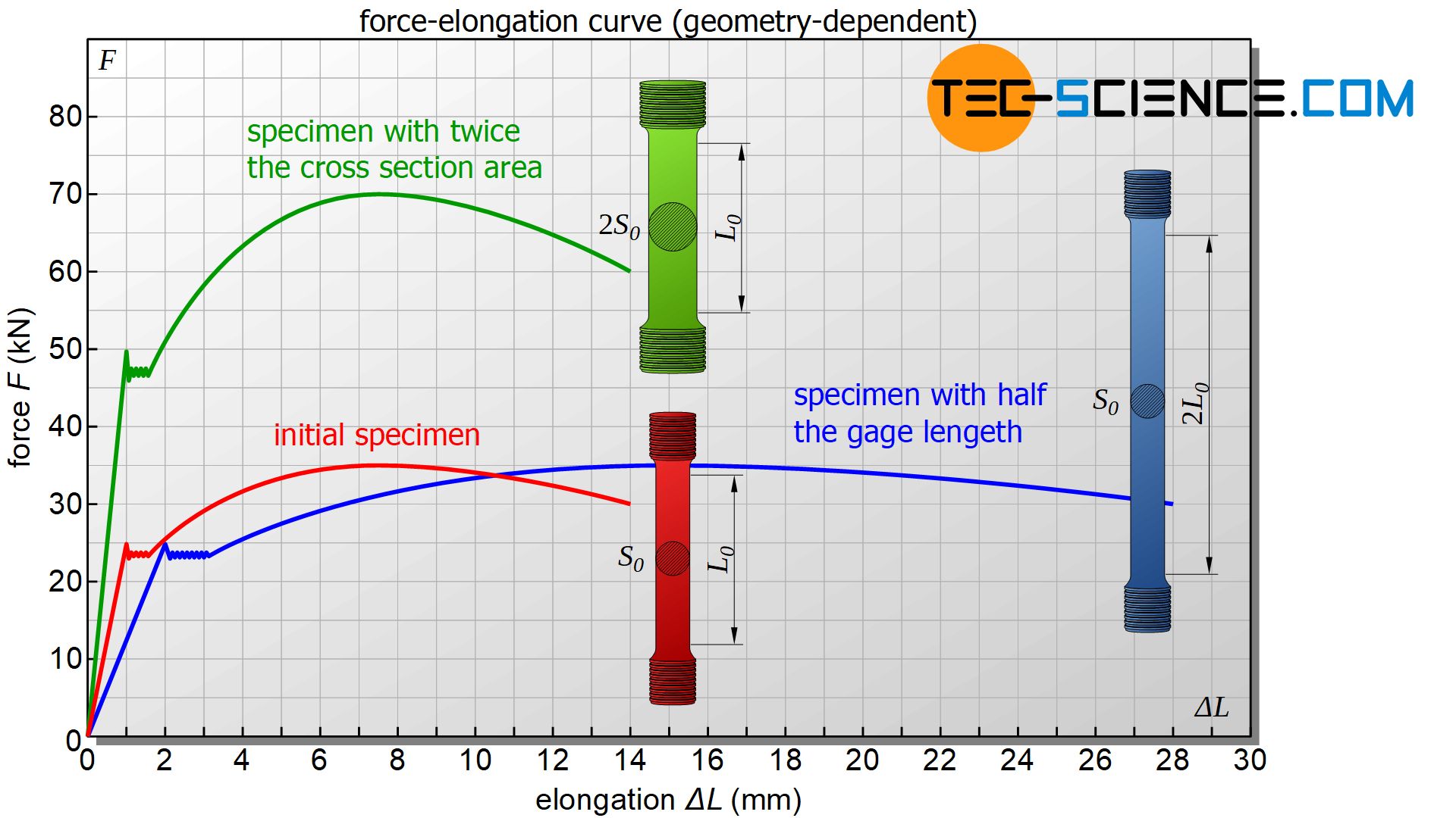
However, such a diagram does not yet allow any statement to be made about the strength of a material! The curve is significantly influenced by the specimen geometry. For example, a thick wood sample may be able to withstand a much greater force than a thin steel sample, provided the wood sample cross-section is much larger than the steel sample cross-section (see green curve). However, this does not mean that wood is generally more resistant to stress than steel.
Stress
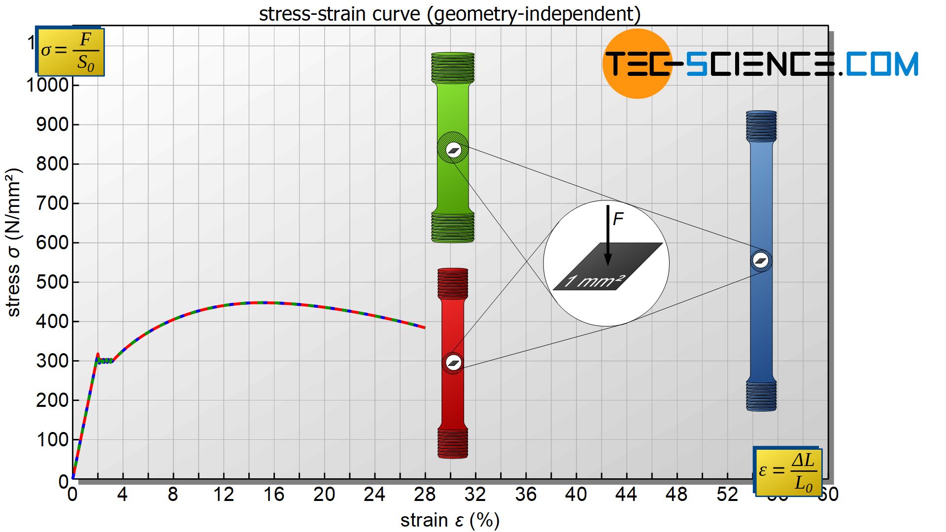
For this reason, the force must be related to an identical cross-sectional area. For practical reasons, it is always advisable to state the force standardized to an area of 1 square millimetre (“Newton per square millimetre”). This means nothing else than to determine the quotient of applied force \(F\) (N) and cross-sectional area \(S_0\) (mm²).
The initial cross-section area \(S_0\) of the specimen always serves as the sectional area, regardless of how it changes in the further course of deformation! This quantity is also called engineering stress \(\sigma\) and is a geometry-independent measure of the load on a material. Thus, independently of the actual cross-sectional area, a comparable statement on the load intensity is obtained when specimens with different cross-sections are stressed in the tensile test.
\begin{align}
\label{technische_spannung}
&\boxed{\sigma = \frac{F}{S_0}}~~~~~[\sigma]=\frac{\text{N}}{\text{mm²}} &&\text{engineering stress} \\[5px]
\end{align}
Stress is a geometrically independent measure of the intensity of a tensile load!
Strain
The measured elongation of the specimen in the tensile test is also still a geometry-dependent quantity. For example a steel specimen may be considerably greater elongated than a wooden specimen despite the same force, provided that the steel specimen is considerably longer than the wooden sample (see blue curve). However, this does not mean that steel can be stretched more than wood.
For this reason, the elongation of the sample must be related to an identical initial length. It is therefore advisable to specify the elongation of the sample as a percentage, i.e. in relation to the initial length. This means nothing else than to determine the quotient of elongation \(\Delta L\) and initial gage length \(L_0\).
This quantity is also called strain \(\epsilon\) and is a geometry-independent measure of specimen elongation. Thus, a comparable statement about the intensity of the lengthening of a specimen is obtained independently of the initial length. For example, a strain of 4 % of a steel speciman means in principle a lower ductility than an elongation of 10 % of a wooden specimen, regardless of the respective initial lengths.
\begin{align}
\label{dehnung}
&\boxed{\epsilon= \frac{\Delta L}{L_0} \cdot 100 \text{%}}~~~~~[\epsilon]=\text{%} ~~~~~\text{strain} \\[5px]
\end{align}
Strain is a geometry-independent measure of the intensity of a elongation!
Stress-strain curve with pronounced yield strength
In summary, it can be said: To eliminate the influence of the specimen geometry, the force is related to the initial cross-section (stress) and the elongation to the initial length (strain)! In this way, the “purely” material-dependent stress-strain curve is obtained from the mainly geometry-dependent force-elongation diagram.
Since the initial cross-section and the initial gage length are each constant quantities (with which the force-elongation curve is “normalized”, so to speak), the force-elongation curve and the stress-strain curve have the same characteristics.
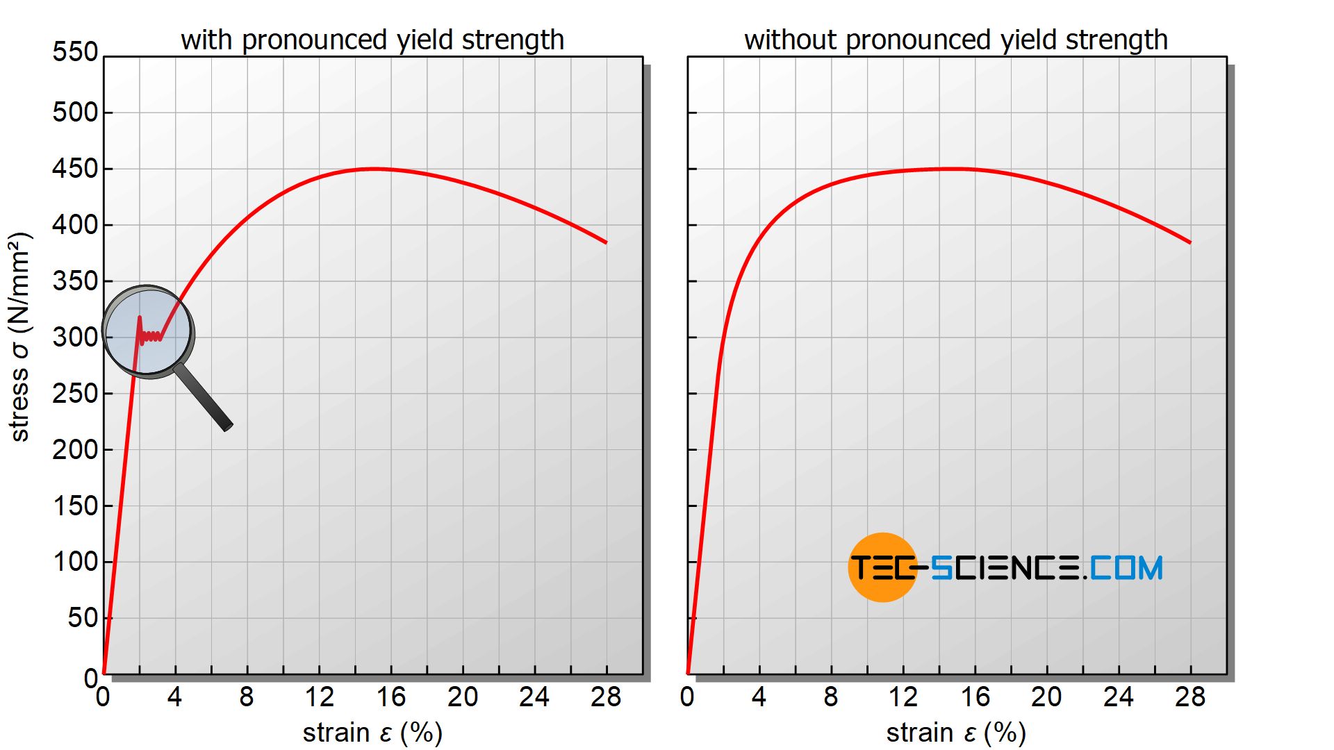
From the stress-strain curve, important parameters about the behaviour of materials under tensile stress can now be obtained. Basically, two different curves can be distinguished for metallic materials, which are explained in more detail in the following sections:
- Stress-strain curve with pronounced yield strength
- Stress-strain curve without pronounced yield strength
In contrast to the force-elongation curve, pure material parameters can be determined from the stress-strain curve which are no longer dependent on the specimen geometry!
Note: In fact, the specimen geometry also plays a role in the stress-strain diagram (even if only a minor one), especially when using different types of tensile test specimen, e.g. round specimen vs. flat specimen. There are also slight differences if a longer specimen (“German” specimen) is used instead of a shorter one (“USA” specimen). Strictly speaking, therefore, comparability of the material parameters is only possible if they were obtained from identical samples.
Elastic strain
For materials with a so-called pronounced yield strength, the figure below shows the typical stress-strain curve. Especially low-carbon steels as well as copper and aluminium alloys show such a typical curve. The diagram can be divided into different regions. Within each region characteristic processes take place in the material, which are described by certain parameters.
First of all, the graph shows a linear increase in which the strain increases in proportion to the applied stress. A doubling of the stress in this region also means a doubling of the strain, or a tripling of the stress also means a tripling of the strain. On this straight line only an elastic deformation takes place. The deformation of the specimen would disappear completely after the force has been removed. Therefore, this region in the diagram is also referred to as elastic region.
Within the elastic region, stress and strain are proportional to each other. Only elastic deformations take place in this region!
Analogous to the elastic range of a spring, this elastic region obeys Hooke’s law. Mechanically loaded components may only be stressed in this leastic range in order to avoid permanent deformation and to guarantee functional reliability in the long term. Think, for example, of cylinder head bolts for engines, where permanent deformation over time would lead to leaks in the cylinder head.
Yield strength (yield point)
The limit to which the material can be elastically stretched without permanent deformation is also called yield strength \(\sigma_y\) or yield point. This strength parameter marks the end of elastic region and can therefore be regarded as the elastic limit. The yield strength can be determined from the tensile force \(F_y\) at the end of the straight line and the initial specimen cross-section \(S_0\):
\begin{align}
\label{streckgrenze}
&\boxed{\sigma_y = \frac{F_y}{S_0}} ~~~~~[R_e]=\frac{\text{N}}{\text{mm²}} ~~~~~\text{yield strength} \\[5px]
\end{align}
The yield strength \(\sigma_y\) indicates the stress limit below which the material undergoes a purely elastic deformation and always reaches its initial length again after removal of the force (elastic limit)! Yield strength is one of the most important material parameters in structural engineering!
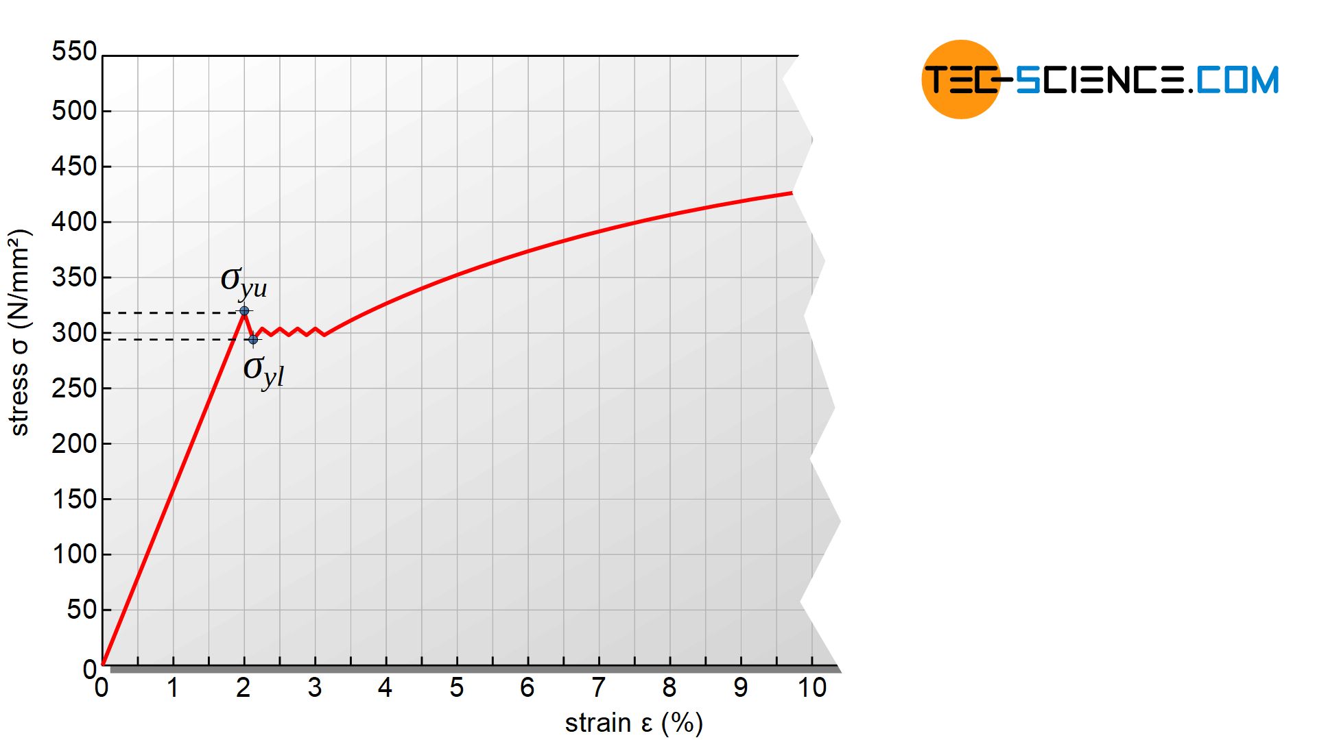
A more precise distinction can be made between the upper yield strength \(\sigma_{yu}\), which marks the beginning of plastic deformation, and the lower yield strength \(\sigma_{yl}\), to which the stress subsequently decreases minimally during the flow of the material (more on this see section yield point elongation).
Elastic modulus
The yield strength is one of the most important strength parameters for the engineer, since it is a decisive factor in determining the strength of a material and thus the functional safety of the construction. Materials for highly stressed screws, for example, should generally have high yield strengths so that they do not deform plastically at high forces.
Although a permanent deformation can be excluded by a sufficient high yield strength, the elastic deformation must still be taken into account. If, for example, screws are stretched too much within the elastic range, the deformation indeed will be completely vanished again after removal of the load, but during operation the screwed parts may be loosened for a short time due to the strong lengthening.
The screws of a pressure vessel, for example, would not be permanently damaged in such a case, but due to the excessive deformation of the screws, the contact pressure between the vessel and the lid would be reduced and tightness would no longer be ensured.

For this reason, the engineer must not only be provided with strength parameters but also deformation parameters. This applies in particular within the elastic range within which most components may only be stressed.
Regarding the stress-strain curve, the aim is therefore to characterize the elastic region, i.e. the quantitative relationship between the applied stress and the resulting strain.
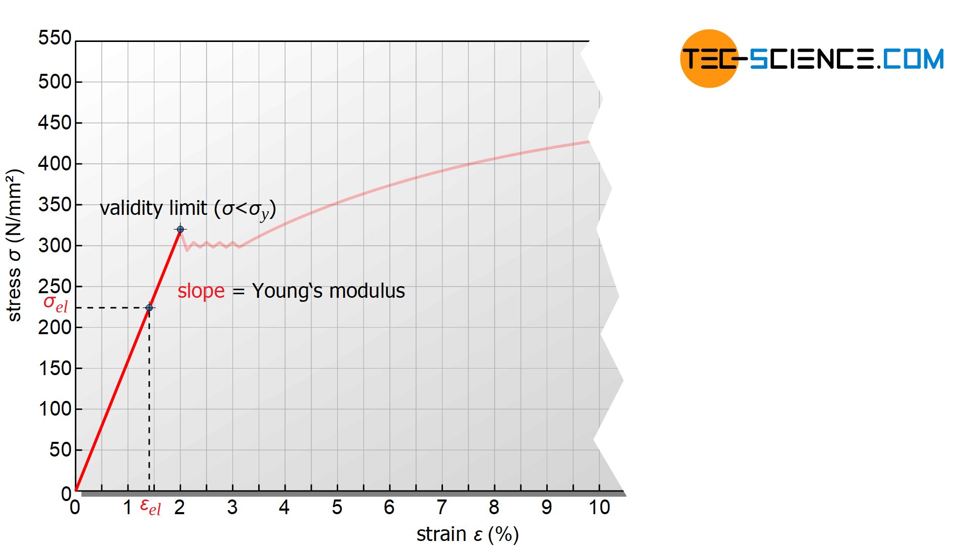
Looking at the straight line, the following qualitative correlation becomes apparent: The steeper the line is, the more stress must be applied for a certain (elastic) strain. Such a material can only be elastically deformed with relatively high forces – it therefore behaves very “stiff”. The slope of the line is therefore a measure of the stiffness of the material and is referred to as the modulus of elasticity or elastic modulus \(E\) (also called Young’s modulus).
For example, guide rods for a high-precision measuring apparatus should have a high stiffness and thus a high Young’s modulus, so that they do not bend too much under their own weight and the weight of the sensor head and thus distort the measuring result.
Since the elastic region of the stress-strain curve is represented by a straight line through the origin, the elastic modulus can be determined relatively easily by dividing stress \(\sigma_{el}\) and strain \(\epsilon_{el}\), whereby the corresponding pair of values must of course be on the straight line. For this reason, the indices “el” are often attached to the respective symbols.
\begin{align}
\label{e_modul}
&\boxed{E = \frac{\sigma_\text{el}}{\epsilon_\text{el}}} ~~~~~[E]=\frac{\text{N}}{\text{mm²}} ~~~~~\text{Young’s modulus} \\[5px]
\end{align}
Note that the modulus of elasticity does not describe the elasticity of a material as one might think from the terminology but exactly the opposite: its stiffness! The higher the modulus of elasticity, the stiffer the material behaves, i.e. less elastic!
An E-module of 210 kN/mm², for example, would theoretically require a stress of 210 kN/mm² to expand the material to twice its original length. Note that the Young’s modulus is actually only valid in the elastic region and specimen elongation to double is only theoretical.
The Young’s modulus is a measure of the stiffness of a material, which describes how much stress is necessary to theoretically stretch the material to twice its initial length!
If the Young’s modulus of a material is determined by the tensile test, then the corresponding strain can be determined for each stress or, conversely, the required stress for each strain. This of course presupposes that the stress is below the yield point and the proportional relationship between stress and strain is given:
\begin{align}
&\boxed{\sigma_\text{el} = E \cdot \epsilon_\text{el}} \\[5px]
\end{align}
Looking at this equation, the analogy to the spring rate is immediately noticeable. While the spring rate \(k\) describes the relationship between force \(F\) and elongation \(ΔL\) as a geometry-dependent quantity, the modulus of elasticity \(E\) characterizes the geometry-independent relationship between the corresponding quantities stress \(\sigma\) and strain \(\epsilon\):
\begin{align}
\label{federhaerte}
F &= k \cdot \Delta L \\[5px]
\sigma_\text{el} &= E \cdot \epsilon_\text{el} \\[5px]
\end{align}
Lüders strain (yield strength elongation)
If the tensile specimen is stretched beyond the elastic limit, the specimen is permanently deformed. The deformation of the specimen would not completely vanish after the force had been removed. This region in the diagram is therefore referred to as the plastic deformation region.
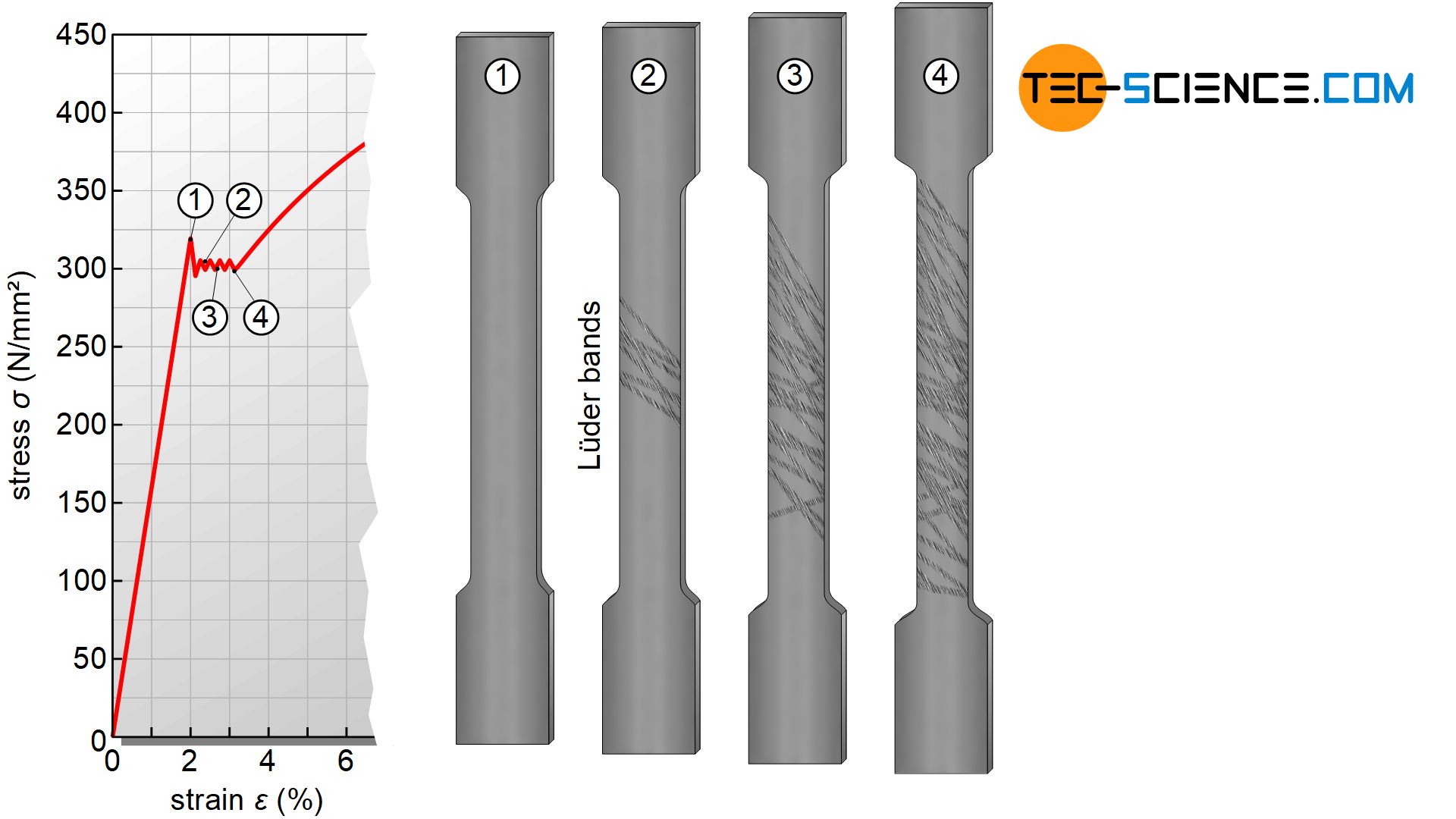
The beginning of plastic deformation is characterized by a short stress drop followed by a small region with almost constant stress, before the stress increases again. In this short range, the sample streches without an increase in stress. Such a curious material behavior is also known as the yield strength effect.
The drop in stress when plastic deformation begins is referred to as yield strength effect!
The cause for the yield strength effect lies in the interaction between accumulations of foreign atoms and dislocations. The inserted half planes of the dislocations create widened zones (dilatation zones) in the area of the dislocation line. In these energetically favourable zones foreign atoms are preferably deposited, whose accumulations are also called Cottrell atmospheres. These foreign atoms initially prevent the dislocations from moving due to their electrostatic forces. This is also referred to as “pinning” of dislocations.

Only at a certain stress, the dislocations can break away from the foreign atoms and the plastic deformation process suddenly begins. Once the dislocations have finally come loose, they only have to be kept moving with less effort. This is accompanied by a reduced force and the stress drops briefly. Only when the dislocations encounter other obstacles will they be pinned again. This explains the short-term drop and the further zigzag-shaped course of the stress-strain curve within a small strain range.
Only when the dislocations have moved through the material and are no longer pinned by Cottrell atmospheres does the stress have to be increased again due to strain hardening in order to achieve further elongation. The region between the onset of plastic deformation (yield strength) and strain hardening is referred to as yield strength elongation or yield point elongation or lüder strain.
Yield strength elongation (Lüders strain) is an inhomogeneous plastic strain at almost constant stress between the beginning of plastic deformation and the onset of strain hardening!
Stretcher strain marks (Lüder bands)
The dislocations emerging during yield point elongation leave visible slip steps. These appear as a matt, strip-shaped network on the shiny surface of the tensile specimen (usually at 45° to the tensile axis). These stretcher strain marks on the surface are also called Lüder bands. In general stretcher strain marks are undesirable in forming technology.
The Lüder strain does not occur evenly or simultaneously over the entire gage length of the tensile specimen but gradually moves from top to bottom or vice versa. This can be seen during the tensile test by the successive Lüder bands, which only gradually cover the entire tensile specimen. The yield point elongation is therefore an inhomogeneous plastic deformation.
Once the tensile test specimen has been stretched beyond the range of the Lüder strain, the yield point effect no longer occurs if the tensile test is repeated in a timely manner. After all, the dislocations have already detached from the Cottrell atmospheres and can move freely from the outset. The elastic deformation then continuously changes into plastic deformation; without yield strength elongation and the associated formation of stretcher strain marks (see also the section below: Stress-strain curve without pronounced yield strength).
For this reason, deep-drawing sheets, which would normally have a yield point effect, are often plastically deformed in advance by rolling. This prevents lüders strain and thus the formation of stretcher strain marks during subsequent deep-drawing. Due to diffusion processes, however, foreign atom accumulations can form again over time, which lead to Cottrell atmospheres – the material ages. In such a case, a yield point effect occurs again.
Portevin–Le Chatelier effect
The yield point effect only occurs at relatively low temperatures. At high temperatures this effect disappears and the stress increases continuously with the strain. The reason for this is the diffusibility of the foreign atoms, which increases strongly at higher temperatures. If the diffusion rate is significantly higher than the dislocation movement, then no accumulations of foreign atoms can form in advance due to the strong particle movement. The dislocations no longer have to tear themselves away from the Cottrell atmospheres and can move freely from the beginning.
A special case arises when the diffusion rate is approximately equal to the velocity of the dislocation. Then the dislocations must tear themselves away from the Cottrell atmospheres, but are captured again by the postdiffusing accumulations of foreign atoms before they have to be torn away from them again. This is noticeable in the stress-strain curve as an increasing zigzag course. Such behavior is also called Portevin-Le-Chatelier effect.
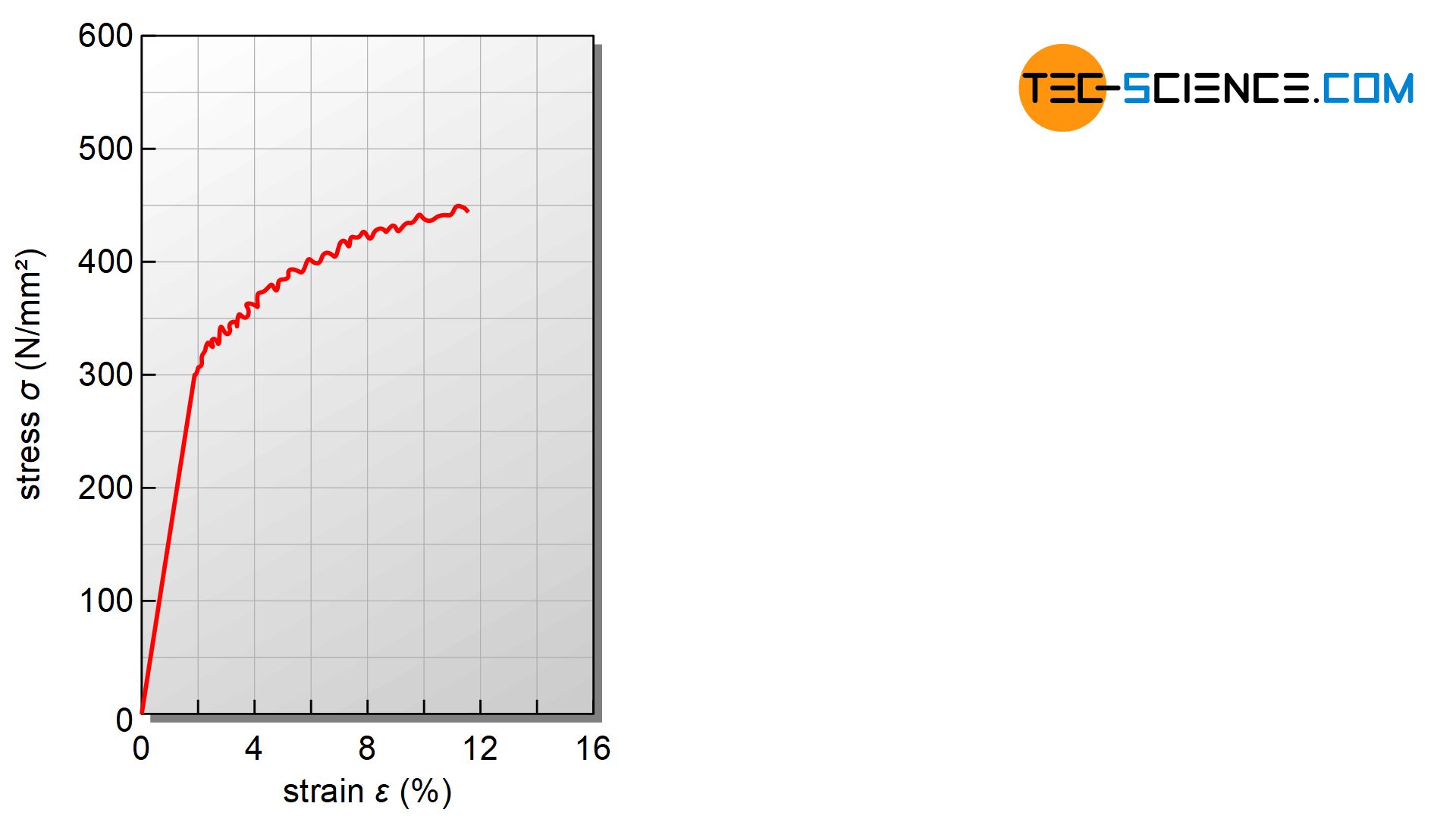
The Portevin-Le-Chatelier effect is a discontinuous increase in stress in the region of lüder strain at elevated temperatures!
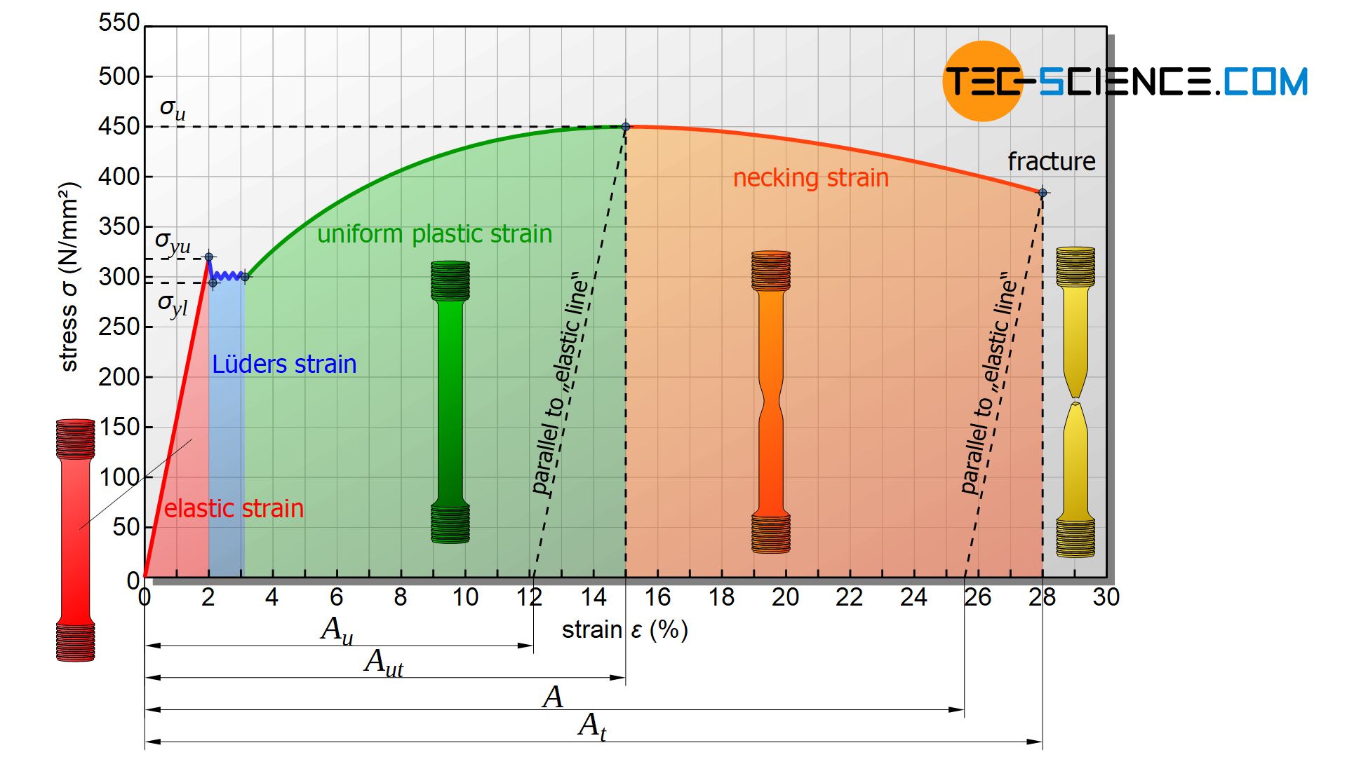
Uniform plastic strain (strain hardening)
After the Lüders strain has been exceeded, the stress must be increased again for a further elongation. In this region the sample stretches very strongly. Since the cross-section of the specimen decreases uniformly over the entire gage length up to the highest point of loading, this strain range is also referred to as the uniform plastic strain (or uniform plastic elongation). In contrast to lüder strain, this is a homogeneous plastic deformation, since the deformation process takes place uniformly over the entire specimen length.
In the region of uniform strain, a noticeable strain hardening of the material occurs. The flattening of the curve to the maximum point is due to the reduction of the specimen cross-section, since the smaller the cross-section, the less force is required to further elongate the specimen. Note that the applied engineering stress is always related to the initial cross-section of the specimen and not to the actual cross-section (see section true stress-strain curve)!
The region of strain hardening in which the tensile specimen is plastically deformed uniformly over the entire length (uniform reduction of the cross-section) is also referred to as uniform strain or uniform elongation!
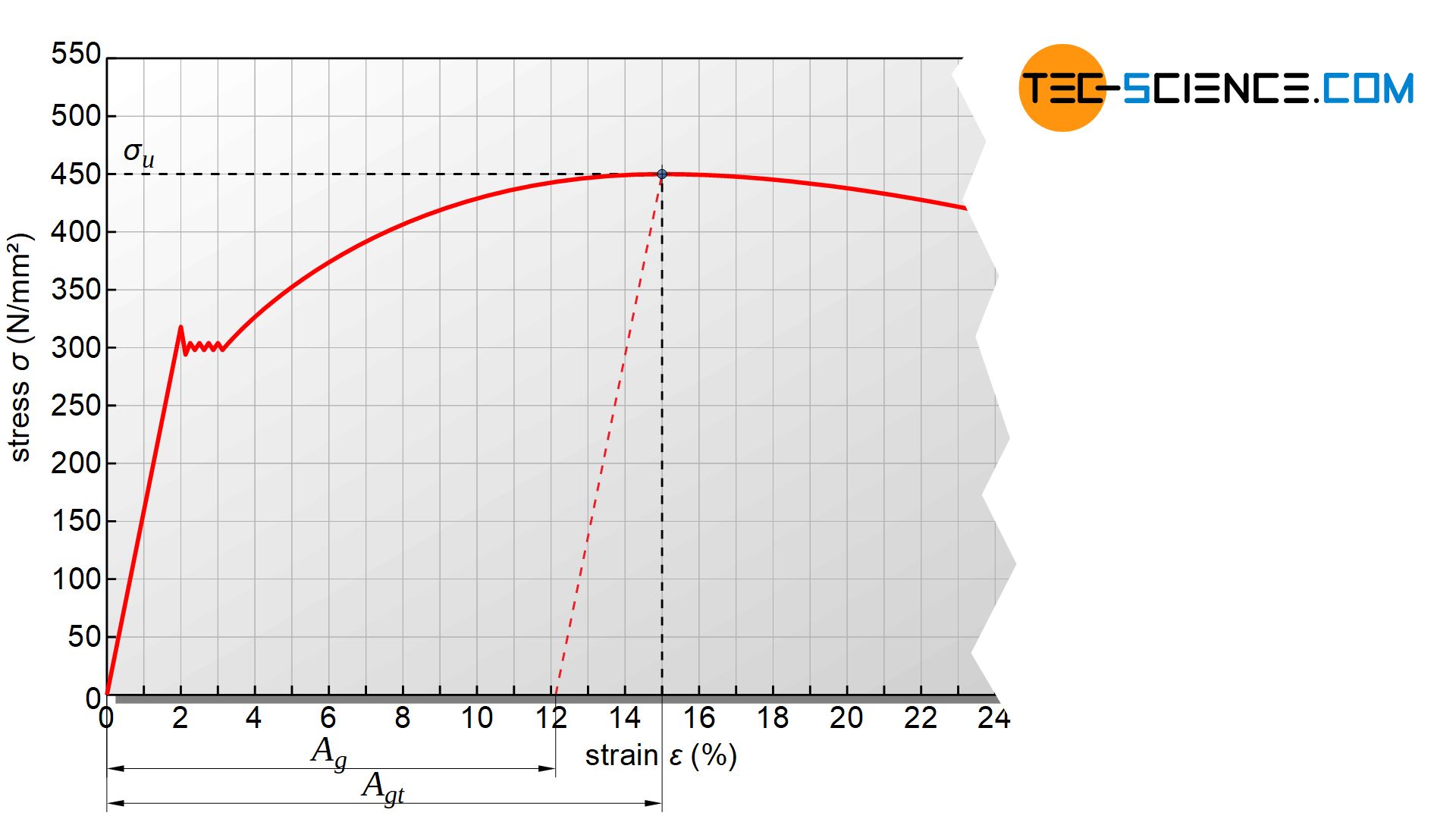
Ultimate tensile strength & uniform strain
Within the uniform strain, the tensile stress rises to a maximum before dropping again. The maximum tensile stress that a material can withstand is called ultimate tensile strength \(\sigma_u\) or just tensile strength. This strength parameter can be determined from the maximum tensile force \(F_u\) and the initial cross-section \(S_0\) of the tensile specimen:
\begin{align}
\label{zugfestigkeit}
&\boxed{\sigma_u = \frac{F_u}{S_0}} ~~~~~[\sigma_u]=\frac{\text{N}}{\text{mm²}} ~~~~~\text{ultimate tensile strength} \\[5px]
\end{align}
Ultimate tensile strength is defined as the maximum stress a material can be subjected to bevor it necks and finally fractures!
The strain that the sample experiences until it reaches tensile strength is called uniform strain( or a bit inaccurate referred to as a uniform elongation). A distinction must be made between whether the specimen is maintained in the state of maximum tensile force or unloaded. If the specimen is relieved, it must be taken into account that the elongation of the specimen decreases again by the proportion of elastic deformation.
Consequently, a distinction can be made between the total uniform strain \(A_{ut}\), which is present as the total strain when the ultimate tensile strength is reached, and the remaining uniform strain \(A_u\), which is actually maintained after the tensile force is removed.
The remaining uniform strain is obtained by shifting the straight line of the elastic region through the maximum of the stress-strain curve. The point of intersection with the horizontal axis then corresponds to the remaining uniform strain. The elastic proportion by which the specimen strain decreases when relieved corresponds to the difference between the two uniform strain values.
The uniform strain range is of particular importance for forming technology. Forming beyond this strain would lead to necking and destroy the material. Therefore, a high uniform strain generally also means good deformation properties.
Uniform strain (uniform elongation) is defined as the strain when the ultimate tensile strength is reached. The greater the uniform strain value, the more pronounced the ability of the material to change its shape without necking!
Yield-tensile ratio
The ratio of yield strength to tensile strength can also be determined as a further parameter from the tensile test. This ratio is called the yield-tensile ratio and is a measure of the risk of breakage by the event of overload:
\begin{align}
\label{streckgrenzenverhaeltnis}
&\boxed{\frac{\sigma_y ~ (\sigma_{y0.2})}{\sigma_u}} ~~~~~\ \text{yield-tensile ratio} \\[5px]
\end{align}
The higher the yield-tensile ratio, the closer the tensile strength and yield strength are to each other. This means that in the event of an overload (exceeding yield strength) there is only a small safety reserve before the material finally necks when the tensile strength is reached and then fractures.
However, the lower the yield-tensile ratio, the greater the difference between tensile strength and yield strength and the greater the safety reserve in the event of overload. However, this also means that the strength of the material can only be used to a small extent. With a yield-tensile ratio of 0.6, for example, only 60% of the maximum stress can be used before the material is plastically deformed. However, this in turn means relatively good ductility of the material, which is important in forming technology. Hardened steels, on the other hand, are hardly formable and therefore achieve yield-tensile ratios of more than 0.95 in some cases.
The yield-tensile ratio is a measure of the risk of fracture when the elastic limit is exceeded!
Necking
When the maximum of the curve (tensile strength) is exceeded, the specimen begins to neck locally. This region of the curve is therefore referred to as the necking region. The stress drop is due to the reduction of the specimen cross-section, since a significantly lower force is required for further elongation with a smaller cross-section. The sample then only elongates within the necking zone until it finally breaks.
In the necking region, the sample locally necks while stress drops until the specimen finally fractures!
Fracture strain (elongation at break)
The remaining strain of the specimen after fracture is called fracture strain \(A\) or somewhat imprecise elongation at break. Again, it must be borne in mind that the specimen is reduced by the proportion of elastic deformation during tearing. To determine this deformation parameter from the stress-strain curve, a parallel line to straight line of the elastic region must be drawn through the fracture point. The intersection with the horizontal axis is then the fracture strain.
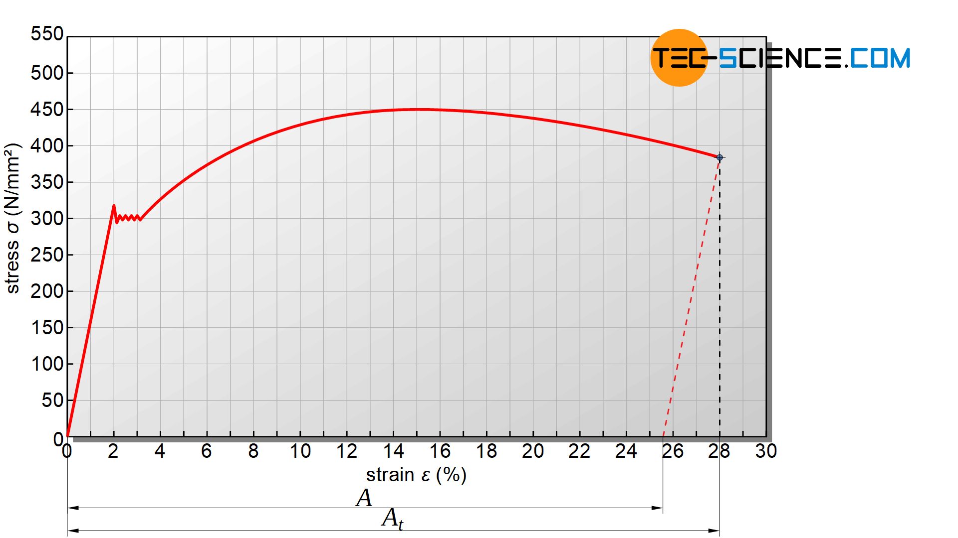
In practice, however, the fracture strain is determined much more precisely by assembling the two fragments and measuring the remaining elongation after fracture \(L_u\). With \(L_0\) as initial gage length, the fracture strain \(A\) is calculated as follows:
\begin{align}
\label{bruchdehnung}
&\boxed{A=\frac{L_u-L_0}{L_0} \cdot 100 \text{%}} ~~~~~[A]=\text{%} ~~~~~\text{fracture strain (elongation at break)} \\[5px]
\end{align}
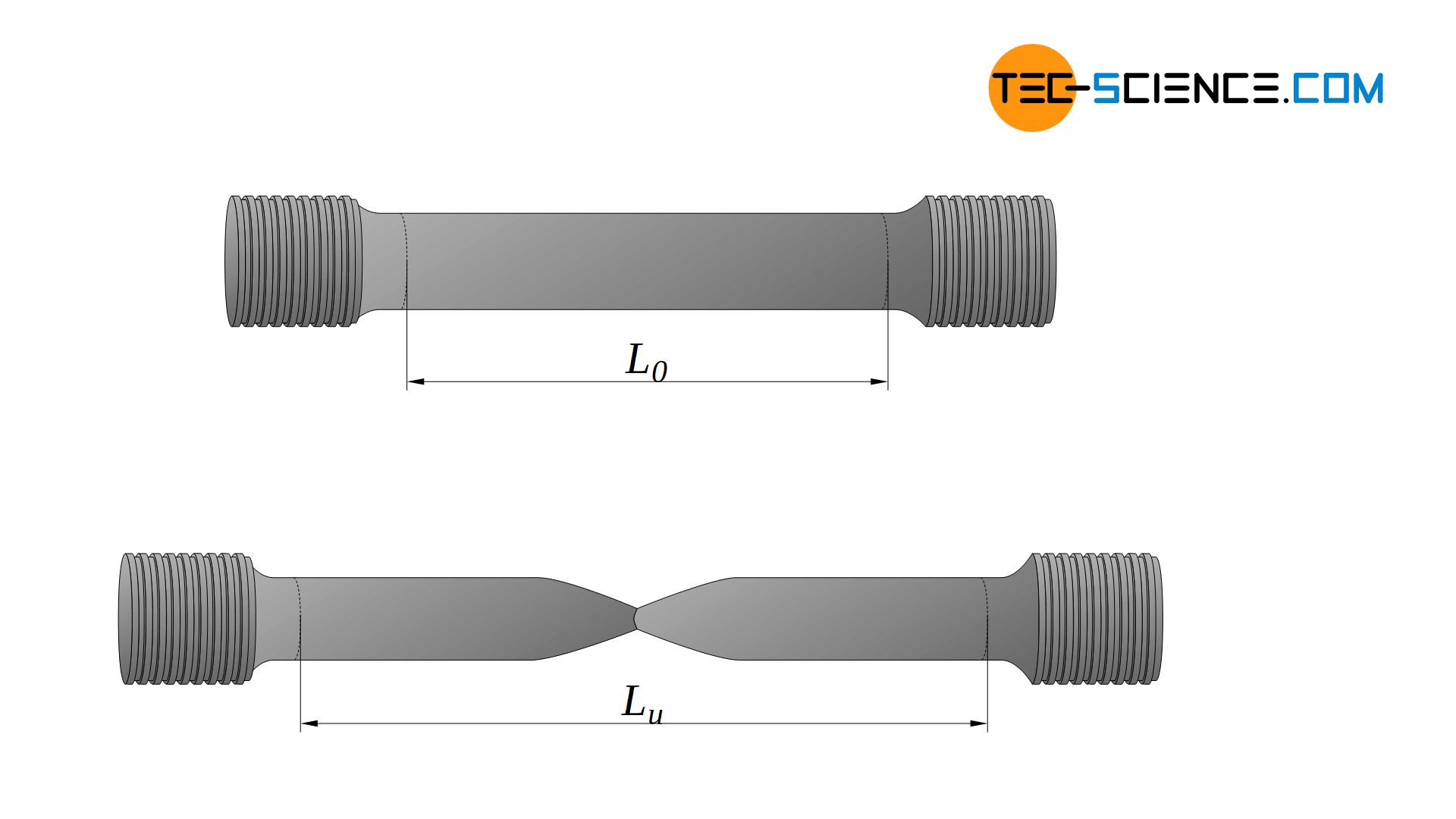
The fracture strain (elongation at break) corresponds to the permanent strain after fracture and is a measure of the deformability of materials!
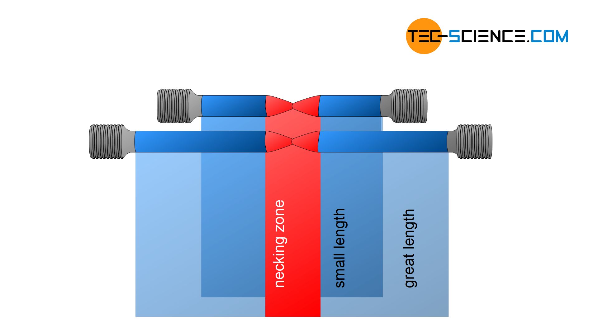
Since tensile specimens elongate only within the necking area when the tensile strength is exceeded, the spatial dimensions of this inhomogeneous strain range are almost identical for both shorter and longer specimens. For short tensile specimens, however, this necking strain accounts for a disproportionately high fraction of the total strain. Tensile tests of a sample with a short gage length therefore always provide higher fracture strain values than tensile tests with greater gage length.
Short tensile specimens show higher fracture strains than longer ones!
Deformation energy
Fracture strain values provide information about the deformation behaviour of materials. Fracture strain plays an important role not only in forming technology but also, for example, in crash-relevant components. For example, bumper beams should absorb as much energy as possible during deformation in the event of an accident. A high fracture strain is an advantage, as this ensures that the component does not break immediately but can absorb as much deformation energy as possible.
In addition to fracture strain, the influence of tensile strength is decisive as well, which also influences the absorption of deformation energy. From the stress-strain curve, the absorbed deformation energy up to fracture can be determined from the area under the curve. Due to the dimension of stress and strain, the area under the curve corresponds to the absorbed energy per unit volume of the material:
\begin{align}
\label{energie}
&\text{Area} = \sigma \cdot \epsilon = \frac{F}{S_0} \cdot \frac{\Delta L}{L_0} = \frac{F \cdot \Delta L}{S_0 \cdot L_0} = \frac{W}{V} = \frac{\text{energy}}{\text{volume}} \\[5px]
\end{align}
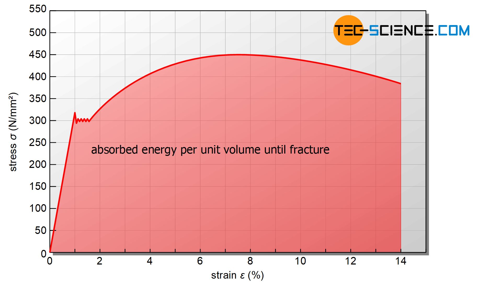
The area under the stress-strain curve corresponds to the energy absorbed per unit volume of the material (energy absorption capacity) until fracture!
Now the stress-strain curve clearly shows that only the combination of high fracture strain and high tensile strength means a very high energy absorption capacity of the material. So-called TRIP light-weight steels (TRansformation Induced Plasticity) have such a property in particular and are therefore frequently used in the automotive industry.
Reduction in area
In addition to fracture strain, the so-called reduction in area \(Z\) also provides information on the deformation behavior of materials. This deformation parameter is determined by the ratio of the reduction in cross-section after fracture and the initial cross-section of the specimen. The reduction in area \(Z\) is thus determined by the smallest specimen cross-section after fracture \(S_u\) and the initial cross-section \(S_0\) as follows:
\begin{align}
\label{brucheinschnuerung}
&\boxed{Z=\frac{S_0-S_u}{S_0} \cdot 100 \text{%}} ~~~~~[Z]=\text{%} ~~~~~\text{reduction in area} \\[5px]
\end{align}
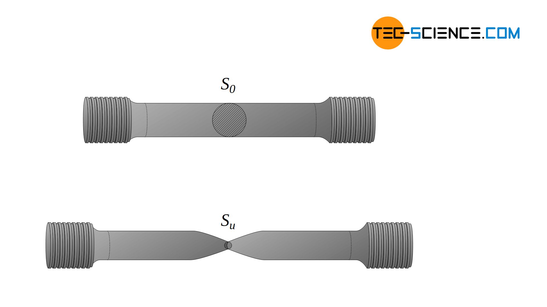
This deformation value descriptively shows, how many percent the cross-section of the specimen has decreased after fracture compared to the initial cross-section. To compensate for uneven deformation, two diameter values at right angles to each other are determined and averaged in order to determine the cross section area after fracture.
A high reduction in area generally means good ductility of the material, while a low value indicates a rather brittle material. Brittle materials are generally undesirable due to their low deformation reserves under overload. Above all because brittle fractures are not announced in advance, for example, by uneven running or loud noises in the machine, due to the (almost) non-existent deformation. Reduction in area can therefore be regarded as a measure of brittle fracture resistance.
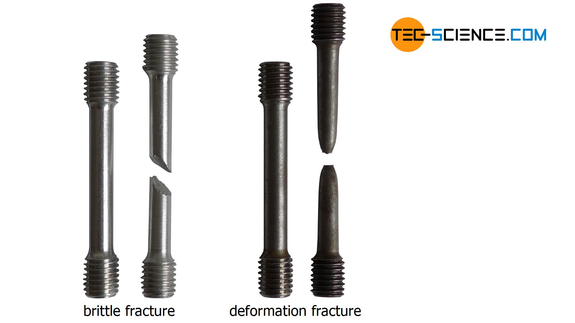
The reduction in area corresponds to the relative decrease of the specimen cross-section after fracture. It is a measure of brittle fracture resistance!
Meaning and application of the parameters
In principle, the deformation parameters such as
- uniform strain,
- fracture strain,
- reduction in area
are not included in calculations for the demensioning of components. In contrast to strength parameters such as
- (offset) yield strength,
- tensile strength and
- modulus of elasticity
the deformation parameters serve only as qualitative characterization in the event of failure. For all characteristic values, it should be noted that comparability for different materials is only given if the values were obtained on identical tensile test specimen geometries and under identical ambient conditions.
| parameter | meaning | application |
|---|---|---|
| yield strength | stress below which the material is subjected to purely elastic stress | highly stressed materials should have highest possible yield strength |
| Young’s modulus | measure of the stiffness of a material (proportionality factor between stress and strain within the elastic region) | materials for components that may only deform slightly (elastically) must have a high modulus of elasticity |
| ultimate tensile strength | maximum loadable stress from which the material necks and finaly fractures | materials for components with high safety relevance must have high tensile strengths |
| yield-tensile ratio | ratio of yield strength to tensile strength. Measure of the risk of fracture if the yield strength is exceeded | materials for safety-relevant components should have the lowest possible yield-tensile ratio |
| offset yield strength | stress at which the material experiences a certain permanent strain | highly stressed materials should have the highest possible offset yield strength (analogous to the yield strength) |
| unifrom strain | measure of the formability of a material without necking | materials for forming technology should have the highest possible uniform strain. |
| fracture strain | measure of the ductility of a material. In combination with a high yield strength, this means a high energy absorption capacity. | materials for components that have to absorb a lot of energy in the event of failure should have a high fracture strain. |
| reduction in area | measure of the brittle fracture resistance of a material | in general, a high reduction in area value of materials is desirable |
Stress-strain curve without pronounced yield strength
In addition to the material behavior under tensile stress presented so far, there are also materials that do not have a pronounced yield strength. This is noticeable in a continuous transition from the elastic region to the plastic region. A yield point is therefore also not clearly visible! For this reason, the stress at which the material remains plastically deformed by 0.2 % is often indicated as the analog limit stress for such materials. This limit stress is then referred to as the 0.2 % offset yield strength \(\sigma_{y0.2}\).
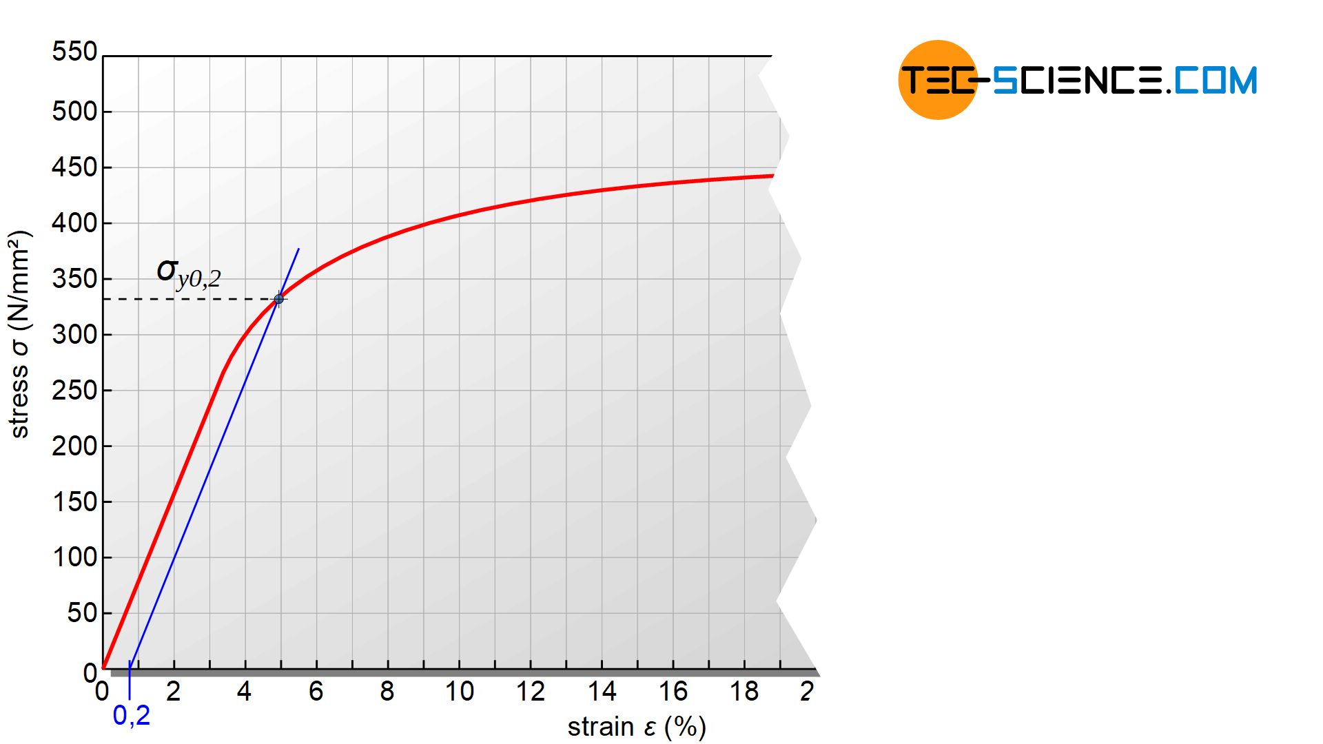
The 0.2 % offset yield strength is obtained graphically by shifting the straight line near the beginning of the curve through the point with 0.2 % strain. The resulting intersection with the stress-strain curve then corresponds to the offset yield strength. In some special cases, a 0.01 % offset yield strength is also used, at which the material then has a permanent strain of 0.01 % ( \(\sigma_{y0.01}\)).
For materials that do not have a pronounced yield strength, an offset yield strength is used, which indicates the stress at a fixed permanent strain!
Note: In contrast to the yield strength at which the material does not undergo any permanent deformation after the force has been removed, the material remains deformed at the offset yield strength!
True stress-strain curve
In the previous analysis, the tensile load was always referred to the initial cross-section of the specimen (“engineering stress”), dispite the fact that it changes in reality (“true stress”). If the force is always related to the actual cross-section of the specimen, the true stress-strain curve is obtained. The diagram below shows the two curves in comparison.
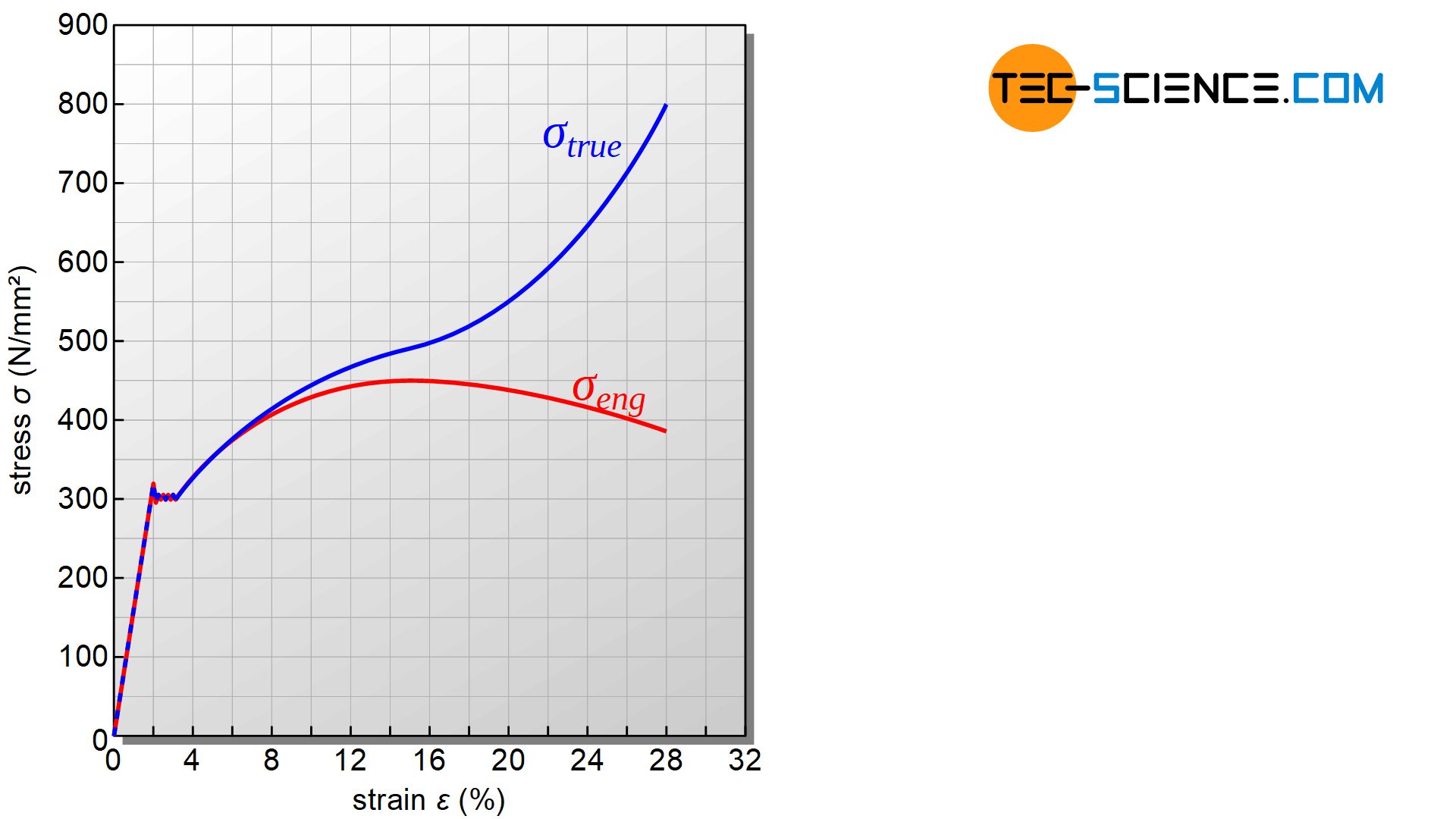
Although the sample cross-section already changes in the elastic range, it does so to such a small extent that both curves initially run almost identically. Only after reaching the yield point do the curves show clearer differences, since the specimen cross-section only decreases significantly in the uniform strain range due to the high elongation and volume constancy. In this region, the true stress increases more than the strain hardening. This is the reason for the strong divergence of the two curves.
This effect is further enhanced by necking. Overall, it becomes obvious that the true stress must be continuously increased in contrast to the engineering stress in order to ultimately fracture the sample. For the egineer, however, the true stress is of no interest, since the dimensioning of components is always based on the undeformed state anyway.


")
")
")