Drag coefficients are dimensionless similarity parameters for describing the drag of flowed around bodies.
Parasitic drag (skin friction drag und pressure drag)
When a body moves through a fluid or a fluid flows around a body, drag forces act on the body. These generally have two causes:
- frictional forces (shear stresses)
- pressure forces (normal stresses)
These two mechanisms have already been explained in detail in the article on Parasitic drag. Therefore, theses mechanisms will only be briefly summarized in the following.
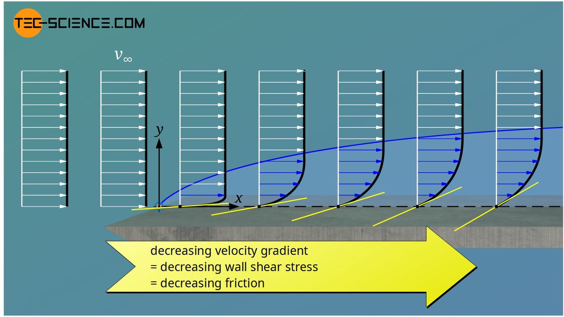
On the one hand, due to the viscosity of the fluid, frictional forces act on the skin of the body, resulting in a so-called skin friction drag. The decisive factor here is the shear stress acting on the surface of the body. These shear stresses are also known as wall shear stresses τw.
Skin friction drag is caused by wall shear stresses that act between the fluid and the body surface due to the viscosity!
On the other hand, the body is affected by different (static) pressure forces. This is a consequence of energy conservation (see Bernoulli’s principle). If a flow around a body accelerates, the static pressure decreases, i.e. the increase in kinetic energy is at the expense of the pressure energy. Conversely, deceleration of the fluid leads to an increase in static pressure at the expense of kinetic energy. The different pressures that arise around the body also lead to a drag. This is also known as pressure drag or form drag.
The pressure drag has its cause in the different static pressures, which act on the body due to the conservation of energy!
Both types of drag (skin friction drag and pressure drag) then form the macroscopically observable drag of a body. This overall drag is also referred to as parasitic drag or just drag.
The sum of skin friction drag and pressure drag is called parasitic drag!
Friction drag, pressure drag and parasitic drag can each be expressed with dimensionless parameters. These quantities are also known as drag coefficients. The meaning of these coefficients is quite analogous to other dimensionless similarity parameters such as Reynolds number, Prandtl number, Nusselt number, Schmidt number, Lewis number, etc.
The drag coefficients serve the purpose of describing flows independently of the size of the system. In this way, for example, the knowledge gained about the drag from a car model in a wind tunnel can be transferred to the real vehicle.
Friction drag coefficient
The friction drag coefficient is used for the characterization of the friction drag which is caused by shear stresses. The friction drag coefficient cf puts the wall shear stress τw in relation to the flow velocity of the undisturbed external flow v∞. The flow velocity is expressed by the dynamic pressure pdyn,∞ of the undisturbed flow. Note that both quantities have the same unit and the quotient is therefore dimensionless. The friction drag coefficient can thus be interpreted as dimensionless wall shear stress.
\begin{align}
\label{cf}
&\boxed{c_f := \frac{\tau_w}{p_{\text{dyn},\infty}}}= \frac{\tau_w}{\tfrac{1}{2}\rho \cdot v_\infty^2} ~~~~~\text{(local) friction drag coefficient}\\[5px]
\end{align}
In this equation, ϱ denotes the density of the fluid. If you take the square root of the quotient of shear stress and density, this quotient also has the dimension of a velocity. This quantity is called shear velocity vτ or friction velocity:
\begin{align}
\label{vw}
&\boxed{v_\tau := \sqrt{\frac{\tau_w}{\rho}}} ~~~~~\text{shear velocity}\\[5px]
\end{align}
The shear velocity is not a velocity in the true sense of the word, it is simply called that because this quantity has the same dimension as a velocity. The shear velocity influences not only the drag coefficient but also the thickness of the viscous sublayer.
The friction drag coefficient can therefore also be determined by the following formula:
\begin{align}
\label{cf2}
&\boxed{c_f = 2 \left(\frac{v_\tau}{v_\infty}\right)^2} \\[5px]
\end{align}
In the case of a flat plate, the growth of the boundary layer is accompanied by a decrease in the velocity gradient at the wall. This results in a decrease of the wall shear stress and thus a reduction of the friction. The friction drag coefficient is therefore by no means a constant quantity, but depends on local conditions.
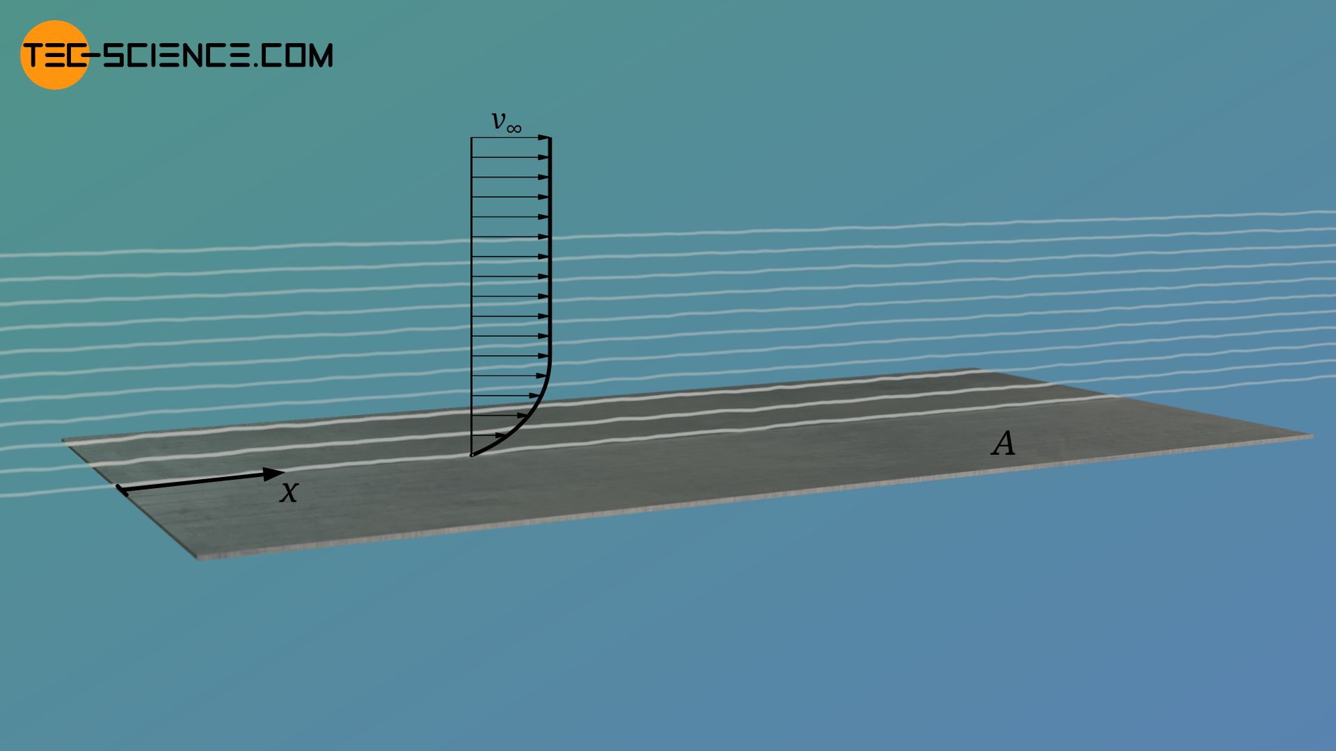
Laminar flow around a plate
For a flat plate and an incompressible laminar flow, the boundary layer equations provide the following relationship between the local Reynolds number at the distance x from the leading edge and the friction drag coefficient there cf,lam (in the formula below, ν denotes the kinematic viscosity of the fluid):
\begin{align}
&\boxed{c_\text{f,lam} = \frac{0.664}{\sqrt{Re_x}}} ~~~~~Re_x = \frac{v_\infty \cdot x}{\nu}~~~~~~~\text{(local friction drag coefficient)}\\[5px]
\end{align}
By integrating the local friction drag coefficients, the overall friction drag coefficient Cf,lam of the entire plate is finally obtained. The (global) Reynolds number in this case refers to the total length of the plate L.
\begin{align}
&\boxed{C_\text{f,lam} = \frac{1.328}{\sqrt{Re_L}}} ~~~~~Re_L = \frac{v_\infty \cdot L}{\nu} ~~~~~~~\text{(overall friction drag coefficient)}\\[5px]
\end{align}
With Cf,lam as the overall friction drag coefficient, the wall shear stress in equation (\ref{cf}) refers to the entire surface area A of the plate (mean wall shear stress τw). Thus, the acting frictional force Ff,lam on this surface can be calculated using the following formula:
\begin{align}
& \overline{\tau}_w = \frac{F_\text{f,lam}}{A} = \frac{1}{2}\rho \cdot v_\infty^2 \cdot C_\text{f,lam} \\[5px]
&\boxed{F_\text{f,lam} = \frac{1}{2}\rho \cdot v_\infty^2 \cdot C_\text{f,lam} \cdot A} ~~\text{flow over a plate}\\[5px]
\end{align}
For a plate with flow around both sides, the frictional force is obviously twice as high, since the frictional force acts on both sides:
\begin{align}
&\boxed{F_\text{f,lam} = \rho \cdot v_\infty^2 \cdot C_\text{f,lam} \cdot A} ~~\text{flow around a plate} \\[5px]
\end{align}
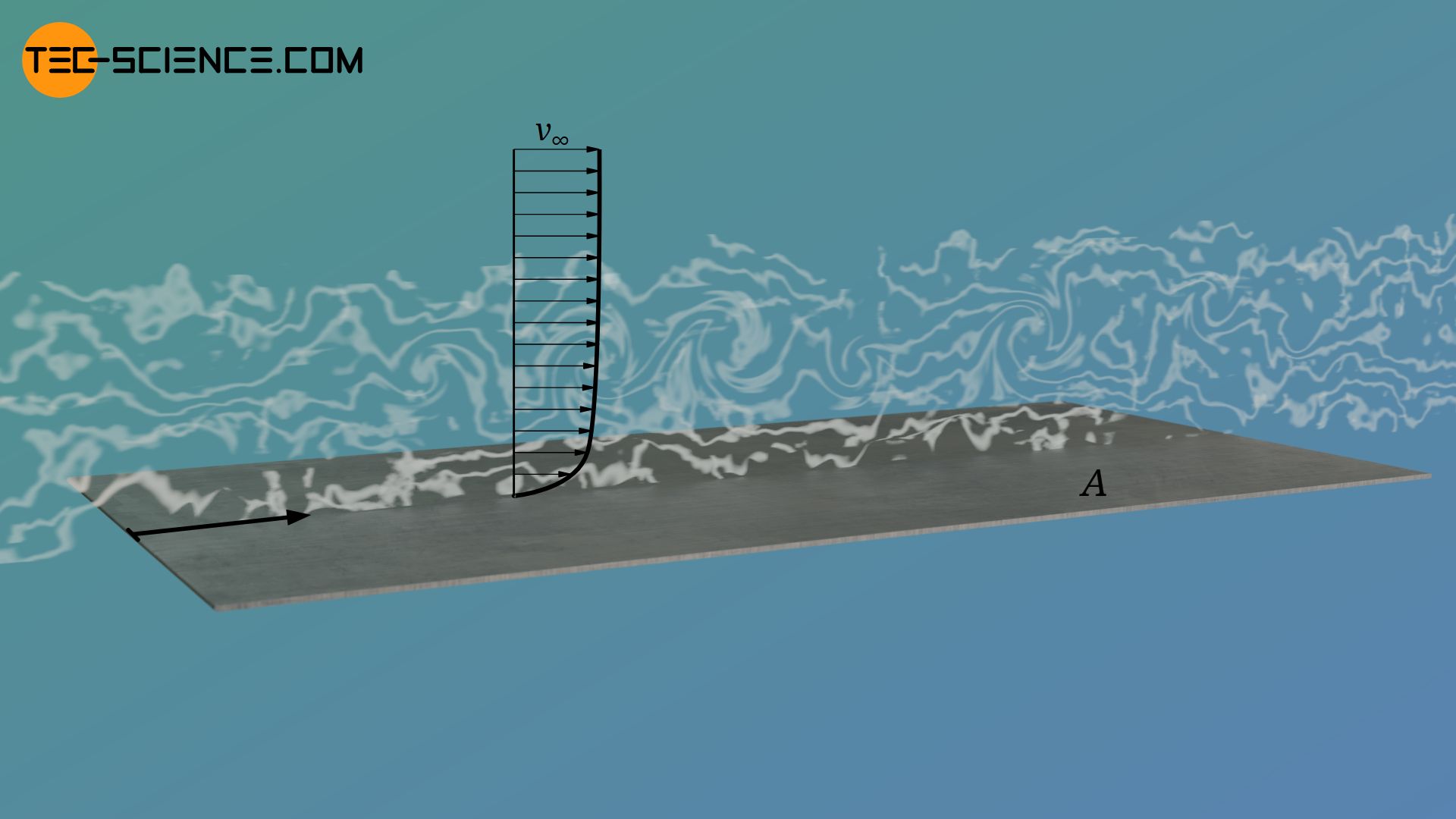
Turbulent flow around a plate
In the article on boundary layers it was shown that the thickness of a laminar boundary layer is inversely proportional to the root of the local Reynolds number:
\begin{align}
&\delta_\text{h,lam} \sim \frac{1}{\sqrt{Re_x}} \\[5px]
\end{align}
This influence is now directly evident in the friction drag coefficients for laminar flow. For a turbulent flow, however, the relationship is the following:
\begin{align}
&\delta_\text{h,tur} \sim \frac{1}{\sqrt[5]{Re_x}} \\[5px]
\end{align}
It can therefore be assumed that the friction drag coefficient of a turbulent flow is influenced in the same way by the local Reynolds number. And indeed, the following relationships apply to the friction drag coefficients:
\begin{align}
&\boxed{c_\text{f,tur} = \frac{0.0577}{\sqrt[5]{Re_x}}} ~~~~~Re_x = \frac{v_\infty \cdot x}{\nu}~~~~~~~\text{(local friction drag coefficient)}\\[5px]
&\boxed{C_\text{f,tur} = \frac{0.0725}{\sqrt[5]{Re_L}}} ~~~~~Re_L = \frac{v_\infty \cdot L}{\nu} ~~~~~~~\text{(overall friction drag coefficient)}\\[5px]
\end{align}
Finally, the frictional force acting on a plate in a turbulent flow can be determined using the following formula:
\begin{align}
&\boxed{F_\text{f,tur} = \frac{1}{2}\rho \cdot v_\infty^2 \cdot C_\text{f,tur} \cdot A} ~~\text{flow over a plate}\\[5px]
&\boxed{F_\text{f,tur} = \rho \cdot v_\infty^2 \cdot C_\text{f,tur} \cdot A} ~~\text{flow around a plate}\\[5px]
\end{align}
Pressure drag coefficient
In the same way as the friction drag coefficient is defined as a dimensionless wall shear stress, the pressure drag coefficient can be defined as a dimensionless (static) pressure difference Δpstat.
\begin{align}
\label{cp}
&\boxed{c_p := \frac{\Delta p_\text{stat}}{p_{\text{dyn},\infty}}} = \frac{p_\text{stat}-p_{\text{stat},\infty}}{\tfrac{1}{2}\rho \cdot v_\infty^2}~~~~~\text{(local) pressure drag coefficient}\\[5px]
\end{align}
In this equation pstat denotes the static pressure at that point where the pressure drag coefficient is to be determined. pstat,∞ is the static pressure in the undisturbed external flow and pdyn,∞ the dynamic pressure. Note that the pressure difference Δpstat is the effective pressure acting on the surface of the object.
For steady, incompressible and frictionless flows, the following relationship applies between a point far away of the plate (undisturbed flow) and any point on the body (see Bernoulli’s principle):
\begin{align}
&p_{\text{stat},\infty}+\tfrac{1}{2}\rho \cdot v_\infty^2 = p_{\text{stat}}+\tfrac{1}{2}\rho \cdot v^2\\[5px]
\end{align}
In this equation, v∞ denotes the flow velocity in the undisturbed flow and v the velocity at any point on the body around which the flow passes. Using this equation, leads to the following formula for calculating the pressure drag coefficient:
\begin{align}
&p_{\text{stat}} – p_{\text{stat},\infty} = \tfrac{1}{2}\rho \cdot v_\infty^2 – \tfrac{1}{2}\rho \cdot v^2 \\[5px]
\label{cpi}
&\boxed{c_p =1- \left(\frac{v}{v_\infty}\right)^2} ~~~\text{applies to frictionless and incompressible flows}\\[5px]
\end{align}
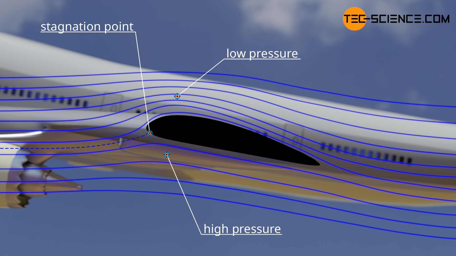
At a stagnation point, kinetic energy of the flow is completely converted into static pressure. This results in a maximum (static) pressure difference (compared to the undisturbed flow). The pressure difference just corresponds to the dynamic pressure of the undisturbed flow and the pressure drag coefficient reaches the maximum value of 1. This can also be seen directly from equation (\ref{cpi}). Since the flow was slowed down to a standstill at the stagnation point (v=0), the pressure drag coefficient is one (cp=1).
However, the pressure drag coefficient can also be zero. In this case, the static pressure at the point under consideration is just as high as the static pressure of the undisturbed flow. Thus there is no pressure difference and the pressure drag coefficient is therefore zero. This can also be seen by means of equation (\ref{cpi}). If the flow is not accelerated or decelerated, then the local flow velocity corresponds to the velocity of the undisturbed flow and the pressure drag coefficient becomes zero.
However, the pressure drag coefficient can also take on negative values. This is the case when a flow alongside a body accelerates (e.g. when air flows over an airfoil). Energy for acceleration is drawn from static pressure. The local static pressure thus decreases. The static pressure difference between the local point and the undisturbed flow is thus negative. This results in negative values for the pressure drag coefficient (this also explains negative pressure upside of an airfoil and resulting lift forces). This too is directly evident from equation (\ref{cpi}). If the local velocity is greater than that of the undisturbed flow, then the quotient of the velocities is greater than 1 and the pressure drag coefficient is negative.
Three cases can therefore be distinguished for incompressible and frictionless flows, which result in characteristic pressure drag coefficients:
| Flow velocity… | increases | decreases | remains constant |
| Pressure drag coefficient | cp<0 | 0<cp<1 | cp=0 |
Note that pressure drag coefficients only describe the dimensionless pressure distribution around a body. Depending on how the surface is directed to the flow, drag forces are generated in different directions. Only those force components that are directed parallel to the flow are decisive for the pressure drag. In general, pressure forces also exist perpendicular to the flow direction. It is exactly these forces which, for example in the case of airfoils, generate a resulting force upwards and give the aircraft lift.
Profile drag coefficient (overall drag coefficient)
As already explained, the sum of viscous drag and pressure drag gives the overall profile drag of a body. This relationship also applies to the drag coefficients. The sum of friction drag coefficient and pressure drag coefficient gives the profile drag coefficient cd of the body.
\begin{align}
\label{ce}
&\boxed{c_d = c_f + c_p} ~~~~~\text{profile drag coefficient} \\[5px]
\end{align}
The profile drag coefficient is sometimes simply called drag coefficient. This relationship of the coefficients can also be derived as follows. Both the wall shear stress τw and the pressure difference Δpstat result formally as force per unit area. By expressing these quantities in terms auf force per unit area, the following formulas apply:
\begin{align}
&c_p = \frac{\Delta p_\text{stat}}{p_{\text{dyn},\infty}} = \frac{F_p}{\frac{1}{2}\rho \cdot v_\infty^2 \cdot A} \\[5px]
&c_f = \frac{\tau_w}{p_{\text{dyn},\infty}} = \frac{F_f}{\frac{1}{2}\rho \cdot v_\infty^2 \cdot A} \\[5px]
\end{align}
The sum of pressure drag force Fp and friction drag force Ff finally gives the overall profile drag force Fd:
\begin{align}
& F_p + F_f = F_d \\[5px]
\end{align}
If this equation is divided by the term ½⋅ϱ⋅v∞2⋅A, the sum of the pressure drag coefficient and the friction drag coefficient is calculated on the left side. The right side of the equation can be interpreted as profile drag coefficient cd:
\begin{align}
& \underbrace{\frac{F_p}{\frac{1}{2}\rho \cdot v_\infty^2 \cdot A}}_{c_p} + \underbrace{\frac{F_f}{\frac{1}{2}\rho \cdot v_\infty^2 \cdot A}}_{c_f} = \underbrace{\frac{F_d}{\frac{1}{2}\rho \cdot v_\infty^2 \cdot A}}_{c_d} \\[5px]
\label{cw}
&\boxed{c_d:=\frac{F_d}{\frac{1}{2}\rho \cdot v_\infty^2 \cdot A}} \\[5px]
\end{align}
As already explained, for streamlined bodies, the profile drag coefficient is mainly determined by the friction drag coefficient. Not only the shape itself is important, but also the angle of attack. For non-streamlined bodies (so-called blunt bodies), or for streamlined bodies with great angles of attack, the pressure drag coefficient mainly influences the profile drag coefficient.
Experimental determination of air resistance
Numerical methods can be used to determine the pressure drag coefficient and the skin friction drag coefficient at the various points of a body and then sum them up to the overall drag coefficient. In most cases, however, it is not necessary to determine the local drag coefficients in such a complicated way, since in practice only the (overall) drag of a body is relevant anyway. This drag can be determined relatively easily in wind tunnels, for example. It is only necessary to measure the drag force that a flow exerts on a body. The quotient of drag force and surface area of the body then corresponds to the drag coefficient (see formula (\ref{cw})).
However, be careful when using the surface area as a basis. Depending on which type of drag dominates, the surface area can refer to the surface projected in direction of flow or to the surface area perpendicular to the flow. In the case of cars or motorcycles, the projected area in direction of the flow has a decisive influence on the drag, since the pressure drag dominates (usually even increased by a flow separation). The projected area corresponds to the area of the shadow on a wall when the body is illuminated in the direction of flow.

However, the projected area has much less influence when a flow flows around a wing of an airplane, because in this case the viscous drag dominates. This drag is largely dependent on the surface area of the wing. The decisive area in this case corresponds to the area of the shadow if the wing is illuminated from above (perpendicular to the flow).

Influence of the Reynolds number on the drag coefficient
The drag coefficient cd depends not only on the shape of a body, but also on the flow velocity v∞, the (characteristic) length L of the body and the kinematic viscosity ν of the fluid. These quantities are represented by the so-called Reynolds number Re:
\begin{align}
&Re=\frac{v_\infty \cdot L}{\nu} \\[5px]
\end{align}
In general, the drag coefficient is therefore a function of the Reynolds number:
\begin{align}
&c_d=c_d(Re) \\[5px]
\end{align}
Since the Reynolds number itself is dependent on the flow velocity, this can lead to the fact that in some situations there is no parabolic relationship between flow velocity and drag. This is the case, for example, in a laminar flows with low flow velocities, where the flow does not separate from the object (see also article Boundary layer separation). In this case the drag coefficient cd decreases almost inversely proportional to the Reynolds number, whereby the drag force Fd formally increases with the square of the velocity. In this case, there is then a linear relationship between flow velocity and drag force:
\begin{align}
&F_d \sim \frac{1}{Re} \cdot v_\infty^2 \sim v_\infty \\[5px]
\end{align}
This linear relationship applies in a very good approximation to Reynolds numbers less than 1, i.e. when the viscosity of the fluid is much greater than the inertial forces of the fluid. This is the case if the fluid is very viscous and the flow velocity is low and the body dimensions are small. For such cases the physicist George Stokes derived a formula to calculate the drag force for spherical bodies (see article Stokes’ law of friction for spherical bodies).
In engineering, when it comes to airflow around cars or airplanes, the Reynolds numbers are generally much higher than 1. In these cases the influence of the Reynolds number on the drag coefficient is very small and the coefficient can be considered almost constant.
Numerical example: We consider a body whose dimension (characteristic length) is in the order of one meter. Air flows around this object at a speed of the order of one meter per second. In this case, one obtains Reynolds numbers in the order of several tens of thousands! If, on the other hand, small particles of the order of a few micrometers in a water flow with a flow velocity of a few centimeters per second were to be observed, then one would obtain Reynolds numbers of the order of 0.01.
This example thus makes it clear that, due to the large Reynolds numbers, a quadratic influence of the flow velocity on the drag force can very often be assumed in practice.
Significance of the quadratic influence of velocity on drag
If a body is moved with a force F and a velocity v, then this body converts the following mechanical power P:
\begin{align}
&P = F \cdot v \\[5px]
\end{align}
In motorized vehicles, this power is supplied by the engine. The force of the engine corresponds exactly to the force required to compensate for the drag force Fd (rolling friction and sliding friction is negligible at high speeds). To overcome the drag (air resistance), the motor must therefore provide the following power:
\begin{align}
&P_d = F_d \cdot v \\[5px]
\end{align}
However, since the drag force increases with the square of the speed, the power increases with the third power of the speed. So doubling the speed of a vehicle means 8 times the engine power required to compensate for drag! This has e.g. enormous effects on the fuel consumption, which is directly related to the engine power. For example, reducing the speed from 140 km/h to 110 km/h would reduce the engine power required to compensate for air resistance by more than half!
In general, a 20% reduction in speed reduces the engine power to compensate for drag by about 50%!
Drag coefficients for selected body shapes
The table below shows the typical drag coefficients for selected bodies. Using the characteristic surface of the body, the drag force for a given flow velocity and density of the fluid can then be determined by using the following formula:
\begin{align}
&\boxed{F_d=\frac{1}{2}\rho \cdot v_\infty^2 \cdot A \cdot c_d } \\[5px]
\end{align}

When objects are moving through resting fluids (e.g. a car or an aeroplane through air), the flow speed then corresponds to the speed of the moving object. The flow velocity thus always corresponds to the relative speed between object and fluid. In the case of air as a fluid, one also speaks in this context of the air resistance.
| Object | Drag coefficient cd |
| Motorcycle | 0.65 |
| Car | 0.35 |
| Bus | 0.45 |
| Truck | 0.5 |
| Human (standing) | 0.8 |
| Ball* | 0.42 (für Re = 70,000) |
| Half hollow sphere (convex side flowed against) | 0.35 |
| Half hollow sphere, “parachute” (concave side flowed against) | 1.35 |
| Airfoil | 0.1 |
| Raindrop (streamlined body) | 0.05 |
| Circular disc | 1.2 |
| Square plate | 0.9 |
| (infinitely) long rectangular plate | 2.0 |
| long thin wire | 1.2 |
*) According to Kaskas, the following formula can be used to determine the drag coefficient of a spherical body in a laminar flow:
\begin{align}
&\boxed{c_d = \frac{24}{Re} +\frac{4}{\sqrt{Re}}+0.4}~~Re<2\cdot 10^5 \\[5px]
\end{align}
Note that for high flow velocities the drag coefficient is asymptotically close to 0.4. For very small Reynolds numbers, however, the last two terms are negligible and Stokes’ law applies:
\begin{align}
&\boxed{c_d = \frac{24}{Re}}~~Re<1 \\[5px]
\end{align}
This then leads to the already mentioned fact that the drag force increases proportionally with speed.
While the direction of flow is obviously not important for a sphere, it is of decisive importance for a hemispherical cup. If the flow hits the open side of the cup, the drag coefficient is almost four times higher than when the flow hits the spherical side. The force that a flow exerts on the cup with the open side in the direction of flow is therefore four times greater. This is used, for example, in so-called hemispherical cup anemometers to generate a defined sense of rotation. The rotational speed is a measure for the wind speed.

")


")
")
