Derivation of the Navier-Stokes equations

The Navier-Stokes equations are used to describe viscous flows. Learn more about the derivation of these equations in this article.

Euler equation

In the article Derivation of the Euler equation the following equation was derived to describe the motion of frictionless flows:

\begin{align}
&\boxed{\frac{\partial \vec v}{\partial t} + \left(\vec v \cdot \vec \nabla \right) \vec v + \frac{1}{\rho} \vec \nabla p = \vec g}~~~\text{Euler equation} \\[5px]
\end{align}

The assumption of a frictionless flow means in particular that the viscosity of fluids is neglected (inviscid fluids). In practice, however, every fluid has a viscosity (even ideal gases!). The viscosity leads to frictional forces within the fluid. Taking the viscosity into account in the Euler equation finally leads to the Navier-Stokes equation.

Normal force acting on a fluid element

For the derivation of the Navier-Stokes equations we consider a fluid element and the forces acting on it. At first we will consider only the motion of the fluid in x-direction. The motion of the fluid element is influenced by the pressure forces acting on the front and back surface of the cubic volume element. These pressure forces basically represent normal stresses and are therefore denoted in the following by the Greek symbol σ instead of p. We will see later that in addition to the pressure forces, viscosity-related forces also act perpendicular to the surfaces and contribute to the normal stress.

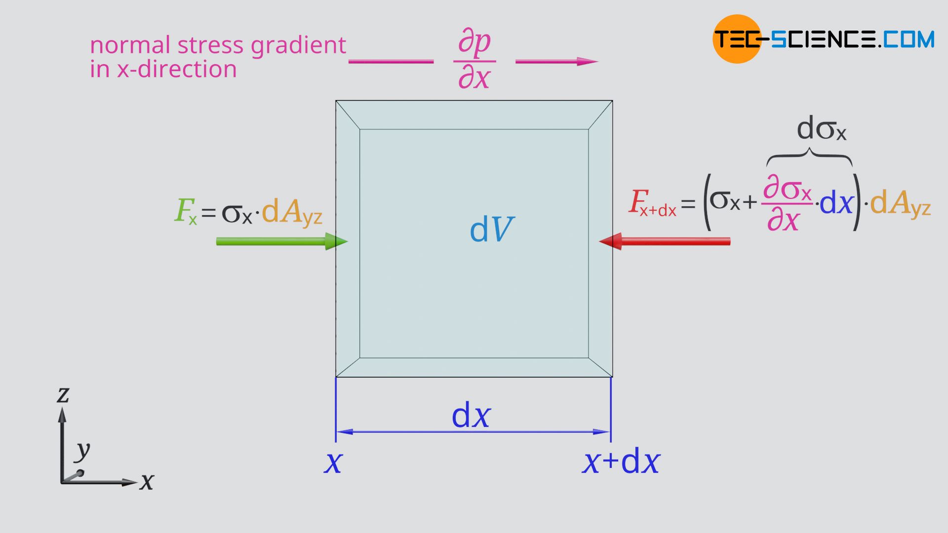
However, the normal stresses acting on the front and back of the fluid element are different, since, for example, the pressure in the direction of flow generally decreases. Thus, a pressure gradient and thus a normal stress gradient ∂σ_x/∂x is present the considered point x. If the normal stress σ_x acts at the position x, then it changes along the distance dx by ∂σ_x/∂x⋅dx. The following pressure-related normal forces thus act at the position x and x+dx on the volume element:

\begin{align}
& \underline{F_\text{x} = \sigma_\text{x} \cdot \text{d}A_\text{yz}} ~~~~~\text{normal force at point }x\\[5px]
& \underline{F_\text{x+dx} = \left(\sigma_\text{x} + \frac{\partial \sigma_\text{x}}{\partial x}\text{d}x\right) \text{d}A_\text{yz}} ~~~~~\text{normal force at point }x+\text{d}x \\[5px]
\end{align}

Since these forces obviously act in different directions, the resulting normal force F_σx on the fluid element is the difference between the two forces:

\begin{align}
\require{cancel}
& F_{\sigma_\text{x}} = F_\text{x} – F_\text{x+dx} \\[5px]
& F_{\sigma_\text{x}} = \sigma_\text{x} \cdot \text{d}A_\text{yz} – \left(\sigma_\text{x}+ \frac{\partial \sigma_\text{x}}{\partial x}\cdot \text{d}x\right) \cdot \text{d}A_\text{yz}\\[5px]
& F_{\sigma_\text{x}} = \cancel{\sigma_\text{x} \cdot \text{d}A_\text{yz}} – \cancel{\sigma_\text{x} \cdot \text{d}A_\text{yz}} – \frac{\partial \sigma_\text{x}}{\partial x} \cdot \underbrace{\text{d}x \cdot \text{d}A_\text{yz}}_{\text{d}V} \\[5px]
& \boxed{F_{\sigma_\text{x}} = ~ – \frac{\partial \sigma_\text{x}}{\partial x} \cdot \text{d}V} ~~\text{resultant normal force in x-direction} \\[5px]
\end{align}

Shear force acting on a fluid element

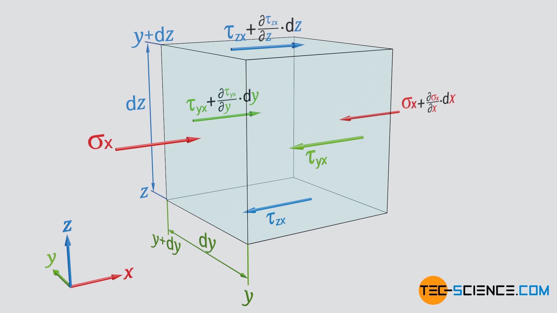
Due to the viscosity η, shear forces or shear stresses in x-direction act on the lateral surfaces of the fluid element and on the top and bottom surfaces. In contrast to the normal stresses considered above, which are directed perpendicular to the surface, the shear stresses act parallel to the surface.

The shear stresses τ_ij are determined according to Newton’s law of fluid friction using the velocity gradient∂v_j/∂i (also called shear rate); more on the validity of this law for a continuum later:

\begin{align}
\label{newton}
& \boxed{\tau_\text{ij} = \eta \cdot \frac{\partial v_\text{j}}{\partial i}} ~~~\text{Newton’s law of fluid friction}\\[5px]
\end{align}

In this equation i (=y,z) denotes the direction of the surface normals for which the shear stress is determined and j (=x) denotes the direction in which the shear stress τ_ij acts. Thus, the designation τ_yx results for the lateral surface at the position y:

\begin{align}
&\underline{\tau_\text{yx}}~~~~~\text{shear stress at point }y \\[5px]
\end{align}

Along the width dy of the fluid element, the velocity gradient ∂v_x/∂y will change in general. Thus, a different shear stress will act at the position y+dy. A corresponding shear stress gradient ∂τ_yx/∂y can be defined at this point so that the following shear stress results at point y+dy:

\begin{align}
&\underline{\tau_\text{yx}+\frac{\partial \tau_\text{yx}}{\partial y}\text{d}y}~~~~~\text{shear stress at point }y+\text{d}y \\[5px]
\end{align}

In concrete terms, a positive shear stress gradient means that according to Newton’s law of fluid friction the velocity gradient increases in the y direction. The flow velocity at the location y+dy is thus greater than at the location y. Looking in the direction of flow (positive x-direction), the fluid flows slower to the right of the fluid element and faster to the left.

The fluid element is slowed down on the right side, so to speak, and on the left side it is carried along by the flow, i.e. accelerated. The shear stress at the point y is thus directed in negative x direction and at the point y+dy in positive direction. The resulting shear stress of the two lateral surfaces is therefore the difference between the two shear stresses:

\begin{align}
&\tau_\text{yx,res} = \underbrace{\tau_\text{yx}+\frac{\partial \tau_\text{yx}}{\partial y}\cdot \text{d}y}_{\text{shear stress at }y+\text{d}y} – \underbrace{\tau_\text{yx}}_{\text{shear stress at }y} \\[5px]
&\underline{\tau_\text{yx,res}=\frac{\partial \tau_\text{yx}}{\partial y}\cdot \text{d}y}~~~~~\text{resultant shear stress on the fluid element} \\[5px]
\end{align}

This shear stress (force per unit area) multiplied by the area dA_xz finally results in the resulting shear force F_τyx acting on the lateral surfaces of the fluid element:

\begin{align}
&F_{\tau_\text{yx}}= \tau_\text{yx,res} \cdot \text{d}A_\text{xz}\\[5px]
&F_{\tau_\text{yx}}=\frac{\partial \tau_\text{yx}}{\partial y}\cdot \underbrace{\text{d}y \cdot \text{d}A_\text{xz}}_{\text{d}V}\\[5px]
\label{for}
&\boxed{F_{\tau_\text{yx}} =\frac{\partial \tau_\text{yx}}{\partial y}\cdot \text{d}V} \\[5px]
\end{align}

For the resulting shear stress or the resulting shear force F_τzx on the top and bottom surface of the fluid element applies quite analogously:

\begin{align}
&\boxed{F_{\tau_\text{zx}} =\frac{\partial \tau_\text{zx}}{\partial z}\cdot \text{d}V} \\[5px]
\end{align}

Weight force acting on a fluid element

In addition to normal and shear forces, gravity generally acts on a fluid element. The considered flow in x-direction does not necessarily have to be horizontal, but can run at any angle. In these cases, only that component of the weight force F_gx is relevant which points in x direction g_x denotes the component of the gravitational acceleration in x direction):

\begin{align}
&F_{\text{g}_\text{x}} = \text{d}m \cdot g_\text{x} \\[5px]
&\boxed{F_{\text{g}_\text{x}} = \rho g_\text{x} \cdot \text{d}V } ~~~\text{weight force on the fluid element in x direction} \\[5px]
\end{align}

In contrast to normal or shear forces (so-called surface forces), the weight force does not act on surfaces, but on the entire “body” of the fluid element. The weight force is therefore a so-called body force. Other body forces acting on the fluid element may be, for example, electrical or magnetic forces. These forces must therefore also be taken into account. At this point, the weight force is therefore only an example of other other forces.

Substantial, local and convective acceleration

The sum of normal force F_σx, shear force F_τyx and F_τzx and body force F_gx finally gives the overall resulting force F_xres acting on the fluid element in x direction:

\begin{align}
&F_{\text{x}_\text{res}} = F_{\sigma_\text{x}} + F_{\tau_\text{yx}} + F_{\tau_\text{zx}} + F_{\text{g}_\text{x}} \\[5px]
&F_{\text{x}_\text{res}} =
– \frac{\partial \sigma_\text{x}}{\partial x} \cdot \text{d}V
+ \frac{\partial \tau_\text{yx}}{\partial y} \cdot \text{d}V
+ \frac{\partial \tau_\text{zx}}{\partial z} \cdot \text{d}V
+ \rho g_\text{x} \cdot \text{d}V
\\[5px]
\end{align}

According to the Newton’s second law, this resultant force leads to the following acceleration a_x in x direction, where dm=ϱ⋅dV denotes the mass of the fluid element:

\begin{align}
\require{cancel}
&a_\text{x} = \frac{F_{\text{x}_\text{res}}}{\text{d}m} = \frac{F_{\text{x}_\text{res}}}{\rho~ \text{d}V} \\[5px]
&a_\text{x} =
\frac{- \frac{\partial \sigma_\text{x}}{\partial x} \cdot \cancel{\text{d}V}
+ \frac{\partial \tau_\text{yx}}{\partial y} \cancel{\text{d}V}
+ \frac{\partial \tau_\text{zx}}{\partial z} \cancel{\text{d}V}
+ \rho g_\text{x} \cdot \cancel{\text{d}V}}{\rho~ \cancel{\text{d}V}}
\\[5px]
&a_\text{x} =
\frac{- \frac{\partial \sigma_\text{x}}{\partial x}
+ \frac{\partial \tau_\text{yx}}{\partial y}
+ \frac{\partial \tau_\text{zx}}{\partial z}
+ \rho g_\text{x}}{\rho}
\\[5px]
\end{align}

Therefore the following equation applies:

\begin{align}
\label{a}
&\underline{a_\text{x}~ \rho=
– \frac{\partial \sigma_\text{x}}{\partial x}
+ \frac{\partial \tau_\text{yx}}{\partial y}
+ \frac{\partial \tau_\text{zx}}{\partial z}
+ \rho g_\text{x} }
\\[5px]
\end{align}

The change in velocity of the fluid element in x direction, also called substantial acceleration a_x, can be expressed by the change in velocity over time at a fixed location (local acceleration: ∂v_x/∂t) and on the other hand by the change in velocity due to the change in location of the fluid element (convective acceleration: ∂v_x/∂x⋅v_x + ∂v_x/∂y⋅v_y + ∂v_x/∂z⋅v_z):

\begin{align}
\label{sub}
&\underbrace{~~a_\text{x}~~}_{\text{substantial}\\\text{acceleration}} = \underbrace{\frac{\partial v_\text{x}}{\partial t}}_{\text{local}\\\text{acceleration}} + \underbrace{\frac{\partial v_\text{x}}{\partial x}v_\text{x} + \frac{\partial v_\text{x}}{\partial y}v_\text{y} + \frac{\partial v_\text{x}}{\partial z}v_\text{z}}_\text{convective acceleration} \\[5px]
\end{align}

This relationship between substantial, local and convective acceleration is described in detail in the article Derivation of the Euler equation and will not be explained further here. If the equation for the substantial acceleration (\ref{sub}) is put into equation (\ref{a}), then the following relationship applies:

\begin{align}
\label{nav}
&\boxed{\left(\frac{\partial v_\text{x}}{\partial t} + \frac{\partial v_\text{x}}{\partial x}v_\text{x} + \frac{\partial v_\text{x}}{\partial y}v_\text{y} + \frac{\partial v_\text{x}}{\partial z}v_\text{z}\right) ~ \rho=- \frac{\partial \sigma_\text{x}}{\partial x} + \frac{\partial \tau_\text{yx}}{\partial y} + \frac{\partial \tau_\text{zx}}{\partial z} + \rho g_\text{x}} \\[5px]
\end{align}

Viscous stress tensor

In three-dimensional flow, the velocity or velocity gradient changes in all three directions. Due to the viscosity, the resulting shear stress is no longer only due to the velocity gradient in a certain direction, but also to a velocity gradient perpendicular to it.

This situation is similar to the deformation of a fluid element. Imagine shear forces that deform the fluid element. In this way, inclined surfaces are formed so that the shear forces acting on the surface now affect another spatial dimension. In fact, in fluids, the stresses acting in additional spatial directions are not due to an actual deformation (magnitude of shearing), but to the shear rate.

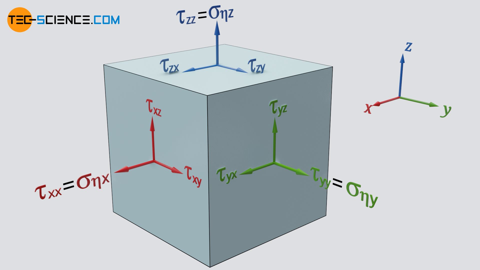
This insight leads to the introduction of a so-called viscous stress tensor, which describes the stresses (normal and shear stresses) acting on a fluid element:

\begin{align}
\label{matr1}
& \boxed{\tau =
\begin{pmatrix}
\color{red}{\tau_\text{xx}} & \tau_\text{xy} & \tau_\text{xz}
\\\
\tau_\text{yx} & \color{red}{\tau_\text{yy}} & \tau_\text{yz}
\\\
\tau_\text{zx} & \tau_\text{zy} & \color{red}{\tau_\text{zz}}
\end{pmatrix}} ~~~\text{viscous stress tensor}\\[5px]
\end{align}

For an isotropic Newtonian fluid, the components of the viscous stress tensor τ can be determined from the viscosity η as follows:

\begin{align}
\label{matr2}
& \boxed{\large\tau = \eta \cdot
\begin{pmatrix}
&\color{red}{\left(\frac{\partial v_\text{x}}{\partial x} + \frac{\partial v_\text{x}}{\partial x}\right)}
& \left(\frac{\partial v_\text{x}}{\partial y} + \frac{\partial v_\text{y}}{\partial x}\right)
& \left(\frac{\partial v_\text{x}}{\partial z} + \frac{\partial v_\text{z}}{\partial x}\right)
\\\
& \left(\frac{\partial v_\text{y}}{\partial x} + \frac{\partial v_\text{x}}{\partial y}\right)
&\color{red}{\left(\frac{\partial v_\text{y}}{\partial y} + \frac{\partial v_\text{y}}{\partial y}\right)}
& \left(\frac{\partial v_\text{y}}{\partial z} + \frac{\partial v_\text{z}}{\partial y}\right)
\\\
& \left(\frac{\partial v_\text{z}}{\partial x} + \frac{\partial v_\text{x}}{\partial z}\right)
& \left(\frac{\partial v_\text{z}}{\partial y} + \frac{\partial v_\text{y}}{\partial z}\right)
&\color{red}{\left(\frac{\partial v_\text{z}}{\partial z} + \frac{\partial v_\text{z}}{\partial z}\right)}
\end{pmatrix}} \\[5px]
\end{align}

The individual entries of the viscous stress tensor can also be determined with the following formula:

\begin{align}
\label{t}
&\boxed{\tau_\text{ij} = \eta \left(\frac{\partial v_\text{i}}{\partial j} + \frac{\partial v_\text{j}}{\partial i}\right)} ~~~\text{viscous stress}\\[5px]
\end{align}

At this point the difference to Newton’s approach according to equation (\ref{newton}) becomes obvious: In three-dimensional flows of a continuum (continuum mechanics) the shear stress depends on a further velocity gradient. This finding and the introduction of the viscous stress tensor is essentially the achievement of Stokes.

For the shear stresses τ_yx and τ_zx in equation (\ref{nav}) applies according to equation (\ref{t}):

\begin{align}
\label{tyx}
&\underline{\tau_\text{yx} = \eta \left(\frac{\partial v_\text{y}}{\partial x} + \frac{\partial v_\text{x}}{\partial y}\right)}\\[5px]
\label{tzx}
&\underline{\tau_\text{zx} = \eta \left(\frac{\partial v_\text{z}}{\partial x} + \frac{\partial v_\text{x}}{\partial z}\right)}\\[5px]
\end{align}

Taking into account the viscous normal stress

For the stresses indicated with identical indices in equation (\ref{matr1}) or (\ref{matr2}) (marked red), both the surface normal and the effective direction of the force obviously point in the same direction. These are therefore not shear stresses but normal stresses, which are often denoted by σ for better differentiation:

\begin{align}
& \tau_\text{xx} = \sigma_{\eta~\text{x}} \\[5px]
& \tau_\text{yy} = \sigma_{\eta~\text{y}} \\[5px]
& \tau_\text{zz} = \sigma_{\eta~\text{z}} \\[5px]
\end{align}

However, this obviously also means that the viscosity generates not only shear stresses but also normal stresses. These normal stresses resulting from the viscosity are therefore additionally designated with the symbol for viscosity η. For the viscosity-related normal stress σ_ηx acting in the x-direction, the following formula (\ref{t}) applies:

\begin{align}
& \tau_\text{xx} =\underline{\sigma_{\eta~\text{x}}}= \eta \left(\frac{\partial v_\text{x}}{\partial x} + \frac{\partial v_\text{x}}{\partial x}\right) = \underline{2\eta \frac{\partial v_\text{x}}{\partial x}} \\[5px]
\end{align}

This viscous normal stress acts as a normal force on the fluid element in addition to the (static) pressure. In contrast to the static pressure, which acts against the surface normal of the fluid element (i.e. is directed towards the fluid element), the viscous normal stress acts in the direction of the surface normal (i.e. away from the fluid element). The resulting normal stress σ_x acting on the fluid element in x-direction thus results from the static pressure p, minus the viscous normal stress σ_ηx:

\begin{align}
& \sigma_\text{x} = p~ – \sigma_{\eta~\text{x}} \\[5px]
\label{sx}
& \underline{\sigma_\text{x} = p~ – 2\eta \frac{\partial v_\text{x}}{\partial x}} \\[5px]
\end{align}

The Navier-Stokes equation for incompressible fluids

If the equations (\ref{tyx}), (\ref{tzx}) and (\ref{sx}) are put into the right side of equation (\ref{nav}), the following equation results (for clarity only the right side of the equation is shown):

\begin{align}
&…=- \frac{\partial \sigma_\text{x}}{\partial x} + \frac{\partial \tau_\text{yx}}{\partial y} + \frac{\partial \tau_\text{zx}}{\partial z} + \rho g_\text{x} \\[5px]

&…=- \frac{\partial}{\partial x}\left(p~ – 2\eta \frac{\partial v_\text{x}}{\partial x}\right) +\eta ~\frac{\partial}{\partial y} \left(\frac{\partial v_\text{y}}{\partial x} + \frac{\partial v_\text{x}}{\partial y}\right) + \eta ~\frac{\partial}{\partial z} \left(\frac{\partial v_\text{z}}{\partial x} + \frac{\partial v_\text{x}}{\partial z}\right)+ \rho g_\text{x} \\[5px]

&…=- \frac{\partial p}{\partial x} + \color{red}{ 2\eta \frac{\partial^2 v_\text{x}}{\partial x^2}} +\eta \frac{\partial}{\partial y} \left(\frac{\partial v_\text{y}}{\partial x}\right) + \eta \frac{\partial^2 v_\text{x}}{\partial y^2}+ \eta \frac{\partial}{\partial z} \left(\frac{\partial v_\text{z}}{\partial x} \right)+ \eta \frac{\partial^2 v_\text{x}}{\partial z^2}+ \rho g_\text{x} \\[5px]
\end{align}

We can also write the term marked in red in a slightly different way:

\begin{align}
…=&- \frac{\partial p}{\partial x} + \color{red}{\eta \frac{\partial^2 v_\text{x}}{\partial x^2} +\eta \frac{\partial}{\partial x} \left(\frac{\partial v_\text{x}}{\partial x}\right)} +\eta \frac{\partial}{\partial y} \left(\frac{\partial v_\text{y}}{\partial x}\right) + \eta \frac{\partial^2 v_\text{x}}{\partial y^2} \\[5px]&
+ \eta \frac{\partial}{\partial z} \left(\frac{\partial v_\text{z}}{\partial x} \right) + \eta \frac{\partial^2 v_\text{x}}{\partial z^2}+ \rho g_\text{x} \\[5px]
\end{align}

Now we rearrange this equation:

\begin{align}
…=&- \frac{\partial p}{\partial x}
+ \eta \left(\frac{\partial^2 v_\text{x}}{\partial x^2}
+ \frac{\partial^2 v_\text{x}}{\partial y^2}
+ \frac{\partial^2 v_\text{x}}{\partial z^2}\right)\\[5px]&
+ \eta \frac{\partial}{\color{red}{\partial x}} \left(\frac{\partial v_\text{x}}{\color{blue}{\partial x}}\right)
+ \eta \frac{\partial}{\color{red}{\partial y}} \left(\frac{\partial v_\text{y}}{\color{blue}{\partial x}}\right)
+ \eta \frac{\partial}{\color{red}{\partial z}} \left(\frac{\partial v_\text{z}}{\color{blue}{\partial x}} \right)
+ \rho g_\text{x} \\[5px]
\end{align}

We can also swap the coordinates of the partial derivatives, because it makes no difference, if we first derive with respect to y and then x or first derive with respect to x and then y. Thus we swap the red marked operators outside the brackets with the blue marked operators inside the brackets:

\begin{align}
…=&- \frac{\partial p}{\partial x}
+ \eta \left(\frac{\partial^2 v_\text{x}}{\partial x^2}
+ \frac{\partial^2 v_\text{x}}{\partial y^2}
+ \frac{\partial^2 v_\text{x}}{\partial z^2}\right)\\[5px]&
+ \eta \frac{\partial}{\color{red}{\partial x}} \left(\frac{\partial v_\text{x}}{\color{blue}{\partial x}}\right)
+ \eta \frac{\partial}{\color{red}{\partial x}} \left(\frac{\partial v_\text{y}}{\color{blue}{\partial y}}\right)
+ \eta \frac{\partial}{\color{red}{\partial x}} \left(\frac{\partial v_\text{z}}{\color{blue}{\partial z}} \right)
+ \rho g_\text{x} \\[5px]
\end{align}

Now we factor out the operator ∂/∂x and the viscosity η:

\begin{align}
…=&- \frac{\partial p}{\partial x}
+ \eta \left(\frac{\partial^2 v_\text{x}}{\partial x^2}
+ \frac{\partial^2 v_\text{x}}{\partial y^2}
+ \frac{\partial^2 v_\text{x}}{\partial z^2}\right)
+ \eta \frac{\partial}{\partial x}
\color{red}{\underbrace{\left(
\frac{\partial v_\text{x}}{\partial x}
+\frac{\partial v_\text{y}}{\partial y}
+\frac{\partial v_\text{z}}{\partial z}
\right)}_{=0}}
+ \rho g_\text{x} \\[5px]
\end{align}

The term marked in red is zero for an incompressible fluid due to the continuity equation (this applies in very good approximation to gases at not too high flow velocities as well)! This simplification finally leads to the following equation, which describes the motion in x direction of an incompressible fluid as a continuum:

\begin{align}
&\left(\frac{\partial v_\text{x}}{\partial t}+ \frac{\partial v_\text{x}}{\partial x}v_\text{x} + \frac{\partial v_\text{x}}{\partial y}v_\text{y} + \frac{\partial v_\text{x}}{\partial z}v_\text{z}\right) \rho
=
– \frac{\partial p}{\partial x}
+ \eta \left(\frac{\partial^2 v_\text{x}}{\partial x^2}
+ \frac{\partial^2 v_\text{x}}{\partial y^2}
+ \frac{\partial^2 v_\text{x}}{\partial z^2}\right)
+ \rho g_\text{x}
\\[5px]
\end{align}

For the motion in y- and z-direction the analogous equations apply. These equations are finally called Navier-Stokes equations:

\begin{align}
&\boxed{\left(\frac{\partial \color{red}{v_\text{x}}}{\partial t}
+ \frac{\partial \color{red}{v_\text{x}}}{\partial x}v_\text{x}
+ \frac{\partial \color{red}{v_\text{x}}}{\partial y}v_\text{y}
+ \frac{\partial \color{red}{v_\text{x}}}{\partial z}v_\text{z}
\right) \rho
=
– \frac{\partial p}{\partial \color{red}{x}}
+ \eta \left(\frac{\partial^2 \color{red}{v_\text{x}}}{\partial x^2}
+ \frac{\partial^2 \color{red}{v_\text{x}}}{\partial y^2}
+ \frac{\partial^2 \color{red}{v_\text{x}}}{\partial z^2}\right)
+ \rho \color{red}{g_\text{x}}}
\\[5px]

&\boxed{\left(\frac{\partial \color{green}{v_\text{y}}}{\partial t}
+ \frac{\partial \color{green}{v_\text{y}}}{\partial x}v_\text{x}
+ \frac{\partial \color{green}{v_\text{y}}}{\partial y}v_\text{y}
+ \frac{\partial \color{green}{v_\text{y}}}{\partial z}v_\text{z}
\right) \rho
=
– \frac{\partial p}{\partial \color{green}{y}}
+ \eta \left(\frac{\partial^2 \color{green}{v_\text{y}}}{\partial x^2}
+ \frac{\partial^2 \color{green}{v_\text{y}}}{\partial y^2}
+ \frac{\partial^2 \color{green}{v_\text{y}}}{\partial z^2}\right)
+ \rho \color{green}{g_\text{y}}}
\\[5px]

&\boxed{\left(\frac{\partial \color{blue}{v_\text{z}}}{\partial t}
+ \frac{\partial \color{blue}{v_\text{z}}}{\partial x}v_\text{x}
+ \frac{\partial \color{blue}{v_\text{z}}}{\partial y}v_\text{y}
+ \text{ }\frac{\partial \color{blue}{v_\text{z}}}{\partial z}v_\text{z}
\right) \rho
=
– \frac{\partial p}{\partial \color{blue}{z}}
+ \eta \left(\frac{\partial^2 \color{blue}{v_\text{z}}}{\partial x^2}
+ \text{ }\frac{\partial^2 \color{blue}{v_\text{z}}}{\partial y^2}
+ \text{ }\frac{\partial^2 \color{blue}{v_\text{z}}}{\partial z^2}\right)
+ \rho \color{blue}{g_\text{z}}}
\\[5px]
\end{align}

In vektorieller Schreibweise stellt sich die Navier-Stokes-Gleichung wie folgt dar:

\begin{align}
&\boxed{ \left[\frac{\partial \vec v}{\partial t} + \left(\vec v \cdot \vec \nabla \right) \vec v \right] \rho = – \vec \nabla p+ \eta \left( \vec \nabla^2 \vec v \right) + \rho \vec g}~~~\text{Navier-Stokes equation} \\[5px]
&\underbrace{\left[\underbrace{\frac{\partial \vec v}{\partial t}}_\text{local acceleration} + \underbrace{\left(\vec v \cdot \vec \nabla \right) \vec v}_\text{convective acceleration} \right]}_\text{(substantial) acceleration} \rho = \underbrace{- \vec \nabla p}_{\text{“pressure force”}\\\text{(normal force)}}+ \underbrace{\eta \left( \vec \nabla^2 \vec v \right)}_{\text{“frictional force”}\\\text{(shear force)}} + \underbrace{\rho \vec g}_{\text{“weight force”}\\\text{(body force)}} \\[5px]
\end{align}

Note that the Navier-Stokes equation shown here only applies to incompressible fluids and approximately also to relatively slow flowing gases!

In general, the Navier-Stokes equations cannot be solved analytically. Only in special cases can a solution or approximate solution be found under simplified assumptions. For example, the special case of an incompressible flow in a pipe results in the law of Hagen-Poiseuille. For fluids for which the viscosity can be neglected (η=0), the Euler equation for inviscid flows is obtained:

\begin{align}
& \left[\frac{\partial \vec v}{\partial t} + \rho \left(\vec v \cdot \vec \nabla \right) \vec v \right] \rho = – \vec \nabla p+ \rho \vec g \\[5px]
&\boxed{\frac{\partial \vec v}{\partial t} + \left(\vec v \cdot \vec \nabla \right) \vec v + \frac{1}{\rho} \vec \nabla p = \vec g}~~~\text{Euler equation} \\[5px]
\end{align}