Derivation of the continuity equation (conservation of mass)

In fluid mechanics, the equation for balancing mass flows and the associated change in density (conservation of mass) is called the continuity equation.

Continuity equation for one-dimensional flows

Experience shows that mass can neither be created out of nothing nor annihilated. Mathematically, this conservation of mass in flows is formulated in the so-called continuity equation.

Mass flux at an finite volume element

To derive the continuity equation we first consider a very small volume element (control volume). The length of the control volume is denoted by Δx and has the width Δy and the height Δz. A compressible fluid flows through this finite volume element. The fluid can enter the volume element through the lateral surfaces and leave it through other surfaces.

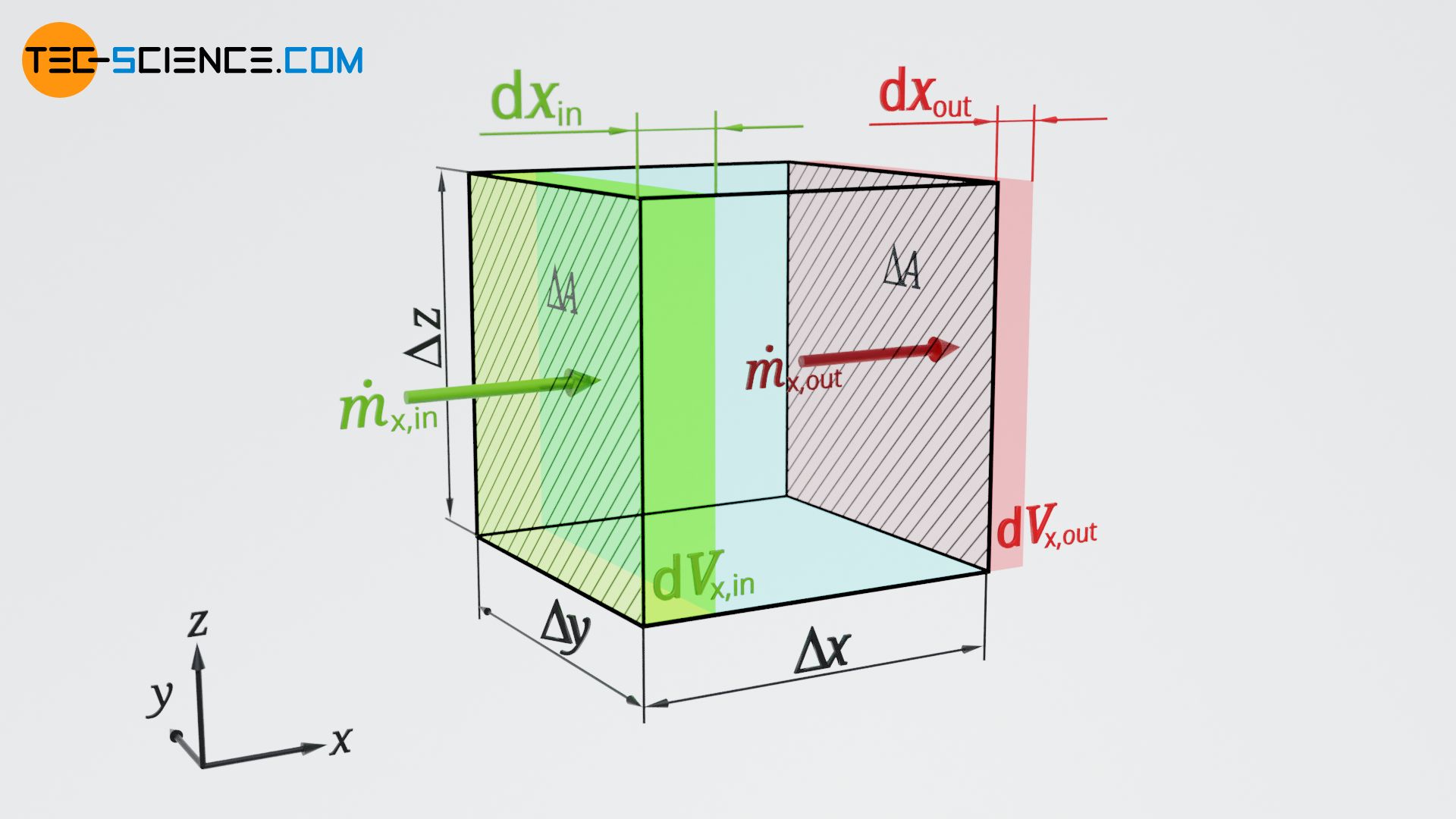
For the sake of simplicity, we will first consider only a flow in the x-direction. Within an infinitesimal time dt a certain mass dm_x,in flows into the volume element. On the opposite side a certain mass dm_x,out leaves the volume element at the same moment.

The inflowing or outflowing mass results from the speed with which the flow enters or leaves the volume element. If the flow enters the volume element with a velocity v_x,in, it travels the infinitesimal distance dx_x,in=v_x,in⋅dt within the time dt. Thus, the following volume dV_x,in flows into the control volume:

\begin{align}
&\text{d}V_\text{x,in}=\Delta A \cdot \text{d}x_\text{x,in} =\Delta A \cdot v_\text{x,in} \cdot \text{d}t\\[5px]
\end{align}

Since we consider an infinitesimal distance dx_x,ein, a constant density can be assumed within the inflowing volume. If the density of the fluid is ϱ_x,in at the point of entry into the volume element, the inflow mass dm_x,in is calculated as follows:

\begin{align}
&\text{d}m_\text{x,in}=\text{d}V_\text{x,in} \cdot \rho_\text{x,in} =\Delta A \cdot \rho_\text{x,in} \cdot v_\text{x,in} \cdot \text{d}t \\[5px]
\end{align}

The mass flowing into the control volume per unit area is therefore only dependent on density and velocity. This area-specific mass flow rate \(\dot m^\text{*}\) is also called mass flux and is marked with an asterisk (*) for better differentiation from the mass flow rate:

\begin{align}
&\dot m_\text{x,in}^\text{*} = \frac{\text{d}m_\text{x,in}}{\Delta A \cdot \text{d}t} = \rho_\text{x,in} \cdot v_\text{x,in} \\[5px]
\label{m_ein}
&\underline{\dot m_\text{x,in}^\text{*} =\rho_\text{x,in} \cdot v_\text{x,in}} \\[5px]
&\boxed{\dot m^\text{*} = \rho \cdot v}~~~\text{mass flux} \\[5px]
\end{align}

The product of density and flow velocity in a flow field of a fluid is called mass flux. It indicates the mass flowing in the flow direction per unit time and unit area!

For compressible fluids, the density in a flow field is generally not constant, but usually differs from one point to another. For example, if the fluid accumulates in the considered control volume, the density and the flow velocity at the outflow of the control volume will differ from the inflow of the control volume. The mass flux at the outflow is calculated in the same way as the mass flux at the inflow [see equation (\ref{m_ein})]:

\begin{align}
&\underline{\dot m_\text{x,out}^\text{*} =\rho_\text{x,out} \cdot v_\text{x,out}} \\[5px]
\end{align}

If more mass flows into the control volume than flows out, the mass inside increases (see animation below). The rate of change of mass \(\dot m_\text{CV}\) in the control volume (CV) results from the difference of the mass flowing in and out (the index x only indicates that the change of the mass in the control volume is due to a flow in x-direction – later on we will consider flow components in y- and z-direction as well):

\begin{align}
\label{m}
& \underbrace{~~\dot m_\text{CV}~~}_\text{change of mass inside the CV} = \underbrace{~~\dot m_\text{x,in}~~}_\text{inflowing mass into the CV} – \underbrace{~~\dot m_\text{x,out}~~}_\text{outflowing mass from the CV} \\[5px]
& \dot m_\text{CV} ~~=~~ \dot m_\text{x,in}^\text{*} \cdot \Delta A~~ -~~ \dot m_\text{x,out}^\text{*} \cdot \Delta A \\[5px]
& \boxed{\dot m_\text{CV} ~~=~~ \dot m_\text{x,in}^\text{*} \cdot \Delta y\cdot \Delta z~~ -~~ \dot m_\text{x,out}^\text{*} \cdot \Delta y \cdot \Delta z} \\[5px]
\end{align}

Mass flux at an infinitesimal volume element

Let us now consider an infinitesimal volume element (control volume) in a compressible flow, where the mass flux and thus the product of density and velocity changes along the x coordinate. Thus, along this x coordinate we can define a gradient of mass flux: ∂(ϱ⋅v_x)/∂x. Over the distance dx (length of the infinitesimal volume element) the following change in mass flux \(\text{d} \dot m_\text{x}^\text{*}\) results in x direction:

\begin{align}
& \underline{\text{d} \dot m_\text{x}^\text{*} =\frac{\partial (\rho v_\text{x})}{\partial x} \cdot \text{d}x} ~~~~~\text{change in mass flux along } \text{d}x \\[5px]
\end{align}

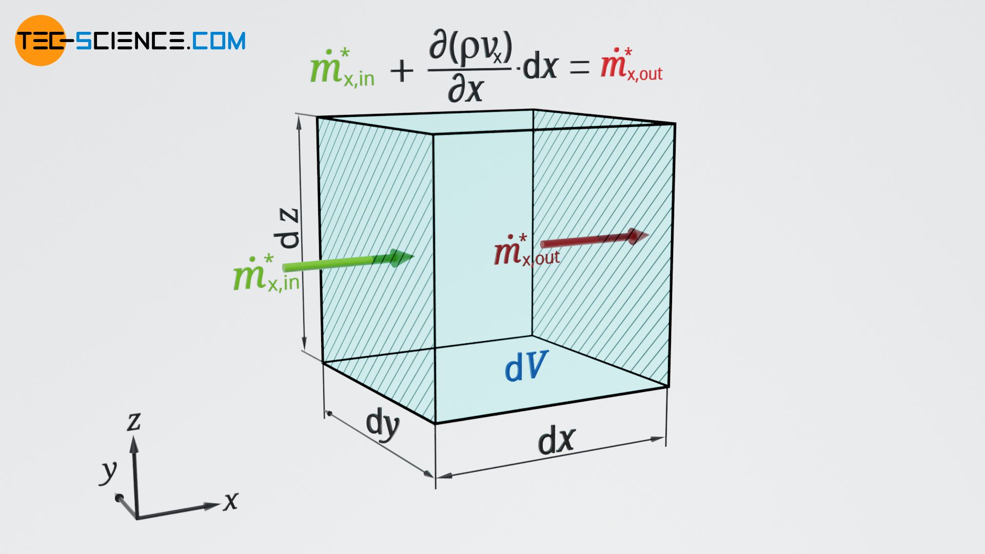
At the outflow of the control volume, the mass flux is thus determined as follows:

\begin{align}
& \dot m_\text{x,out}^\text{*} =\dot m_\text{x,in}^\text{*} +\text{d} \dot m_\text{x} \\[5px]
& \underline{\dot m_\text{x,out}^\text{*} =\dot m_\text{x,in}^\text{*} + \frac{\partial (\rho v_\text{x})}{\partial x} \cdot \text{d}x} ~~~~~\text{outflowing mass flux}\\[5px]
\end{align}

The resulting temporal change of mass \(\dot m_\text{CV}\) inside the control volume can be determined with equation (\ref{m}), whereby the infinitesimal dimensions dy and dz are used at this point:

\begin{align}
\require{cancel}
& \dot m_\text{CV} = \dot m_\text{x,in}^\text{*} \cdot \text{d}y \cdot \text{d}z ~-~ \dot m_\text{x,out}^\text{*} \cdot \text{d}y \cdot \text{d}z \\[5px]
& \dot m_\text{CV} = \dot m_\text{x,in}^\text{*}\cdot \text{d}y \cdot \text{d}z ~-~ \left(\dot m_\text{x,in}^\text{*}+ \frac{\partial (\rho v_\text{x})}{\partial x} \cdot \text{d}x \right) \cdot \text{d}y \cdot \text{d}z \\[5px]
& \dot m_\text{CV} = \cancel{\dot m_\text{x,in}^\text{*}\cdot \text{d}y \cdot \text{d}z} ~-~ \cancel{\dot m_\text{x,in}^\text{*} \cdot \text{d}y \cdot \text{d}z}~-~ \frac{\partial (\rho v_\text{x})}{\partial x} \cdot \text{d}x \cdot \text{d}y \cdot \text{d}z \\[5px]
&\dot m_\text{CV} = ~- \frac{\partial (\rho v_\text{x})}{\partial x} \cdot \underbrace{\text{d}x \cdot \text{d}y \cdot \text{d}z}_{\text{d}V} \\[5px]
\label{a}
&\underline{\dot m_\text{CV} = ~- \frac{\partial (\rho v_\text{x})}{\partial x} \cdot \text{d}V } \\[5px]
\end{align}

The negative sign indicates that in case of a positive gradient the mass in the volume element decreases over time, because obviously the outgoing mass flow is larger than the incoming mass flow. However, if the mass in the volume element generally changes over time, then its density ϱ also changes over time:

\begin{align}
\label{b}
&\underline{\dot m_\text{CV} = \frac{\partial \rho}{\partial t} \cdot \text{d}V} \\[5px]
\end{align}

Note that we are looking at an infinitesimal volume element, to which a single density, changing over time, can be assigned. In the next step, we will see that the size of the volume element does not matter anyway and thus can indeed be chosen infinitesimally small. Furthermore, note that the density in flows generally varies not only over time (e.g. in unsteady flows), but also changes from one point to another (e.g. in a pipe reducer). The temporal change of density is therefore a partial derivative of the density function with respect to time.

Using equation (\ref{b}) in equation (\ref{a}), the following relationship is finally obtained between the gradient of the mass flux and the resulting temporal change of the density in one point of the flow:

\begin{align}
\require{cancel}
&\frac{\partial \rho}{\partial t} \cdot \cancel{\text{d}V} = ~- \frac{\partial (\rho v_\text{x})}{\partial x} \cdot \cancel{\text{d}V} \\[5px]
&\boxed{\frac{\partial \rho}{\partial t} = ~- \frac{\partial (\rho v_\text{x})}{\partial x}}~~~\text{continuity equation for one-dimensional flows} \\[5px]
\end{align}

This equation is finally called continuity equation and is valid in this form for one-dimensional flows. As seen, this equation results from the conservation of mass. The continuity equation serves to determine the temporal change of density in arbitrary points of a flow by means of the existing flow field (represented by the vectors of the mass flux). Thus statements about the development of unsteady flows of compressible fluids are possible. According to the continuity equation, the following statement applies:

The gradient of the mass flux in a point of a flow corresponds to the temporal change of the density in this point!

Note that the mass flux is a vector and points in the same direction as flow velocity, since it is ultimately a product of a vector (velocity) and a scalar (density). The mass flux is basically a flow velocity weighted by the density. To illustrate flow fields, see also the article Streamlines, pathlines, streaklines and timelines.

Continuity equation for three-dimensional flows

The previous consideration was limited to a one-dimensional flow in x-direction. In general, however, a flow is three-dimensional, i.e. the flow velocity has components in all three directions. Therefore, not only the mass flow through a volume element in x direction may be considered, but also the flow components in y and z direction must be taken into account. Mass does not only flow into and out of the volume element through the front and rear surface, but also through the lateral surfaces (y direction) and the bottom and top surface (z-direction).

For the y and z direction, the changes of mass inside the control volume can be determined in the same way as in equation (\ref{a}):

\begin{align}
\label{aa}
&\dot m_\text{x} = ~- \frac{\partial (\rho v_\text{x})}{\partial x} \cdot \text{d}V \\[5px]
\label{c}
&\dot m_\text{y} = ~- \frac{\partial (\rho v_\text{y})}{\partial y} \cdot \text{d}V \\[5px]
\label{d}
&\dot m_\text{z} = ~- \frac{\partial (\rho v_\text{z})}{\partial z} \cdot \text{d}V \\[5px]
\end{align}

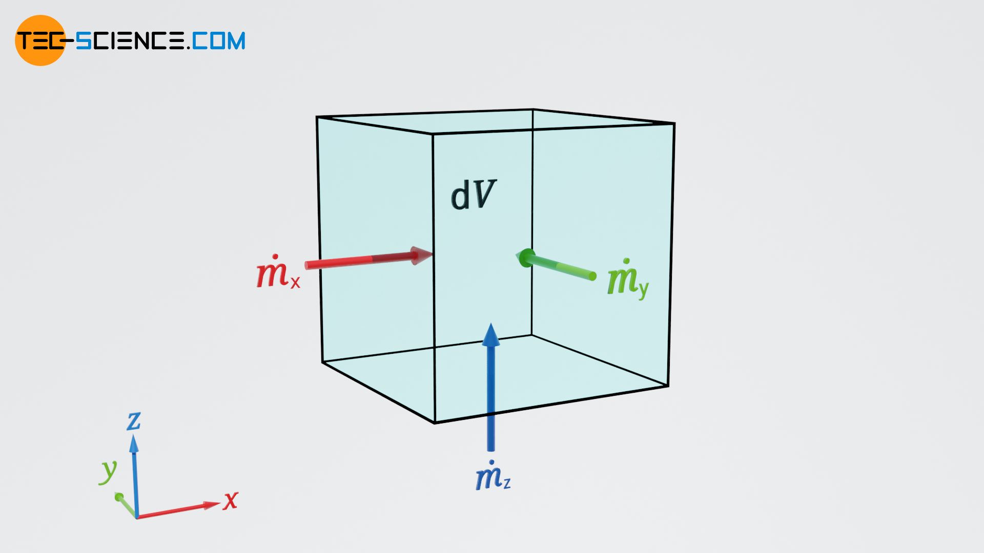
In this equation the velocities v_x, v_y and v_z denote the components of the flow vector v. The resulting change in mass in the infinitesimal control volume is now no longer only due to a flow in x direction, but also to the flow components in y and z direction. As with equation (\ref{b}) for a one-dimensional flow, the following formula now applies to a three-dimensional flow:

\begin{align}
&\underbrace{\frac{\partial \rho}{\partial t} \cdot \text{d}V}_\text{change in mass inside the control volume} = \underbrace{\dot m_\text{x}+\dot m_\text{y} +\dot m_\text{z}}_{\text{mass flowing over the boundaries of the control volume}} \\[5px]
\end{align}

Equations (\ref{aa}) to (\ref{d}) used in this equation finally provides the continuity equation for three-dimensional flows:

\begin{align}
\require{cancel}
&\frac{\partial \rho}{\partial t} \cdot \cancel{\text{d}V}= ~- \frac{\partial (\rho v_\text{x})}{\partial x}\cdot \cancel{\text{d}V} – \frac{\partial (\rho v_\text{y})}{\partial y}\cdot \cancel{\text{d}V} – \frac{\partial (\rho v_\text{z})}{\partial z}\cdot \cancel{\text{d}V} \\[5px]
&\boxed{\frac{\partial \rho}{\partial t} = ~- \left[\frac{\partial (\rho v_\text{x})}{\partial x}+ \frac{\partial (\rho v_\text{y})}{\partial y}+ \frac{\partial (\rho v_\text{z})}{\partial z}\right]}~~~\text{continuity equation} \\[5px]
\end{align}

The sum of the partial derivatives with respect to the different directions (sum of the gradients of mass flux) is also called divergence (div) in mathematics. The divergence is a mathematical operator, which balances flows through a volume element in case of a flow field. The divergence can also be written as scalar product of del operator ∇ and vector field of mass flux ϱv:

\begin{align}
&\boxed{\frac{\partial \rho}{\partial t} = ~- \text{div}\left(\rho \vec v \right) }~~~\text{where}~~~\text{div}\left(\rho \vec v \right) = \vec \nabla \cdot \rho \vec v =\frac{\partial (\rho v_\text{x})}{\partial x}+ \frac{\partial (\rho v_\text{y})}{\partial y}+ \frac{\partial (\rho v_\text{z})}{\partial z} \\[5px]
\end{align}

For incompressible fluids the density does not change and is therefore constant over time. The partial derivative of the density with respect to time is therefore zero (∂ϱ/∂t=0). Furthermore, the density is also spatially constant and can therefore be written before the divergence operator. For incompressible fluids, the continuity equation has therefore the following form:

\begin{align}
&\boxed{\text{div}\left(\vec v \right) = 0} ~~~\text{continuity equation for incompressible fluids} \\[5px]
\end{align}

Interpretation of the divergence

Vector fields can be visualized with arrows. The length of the arrows indicates the magnitude of the quantity and the arrowheads show the direction. Vector fields can also be visualized by field lines. The density of the field lines indicate the magnitude of the field strength and the tangent to the field lines show the direction. In a similar way the flow field of fluids can be visualized by streamlines (“field lines”). The density of the streamlines is a measure for the flow velocity and the tangent to the streamlines show the flow direction.

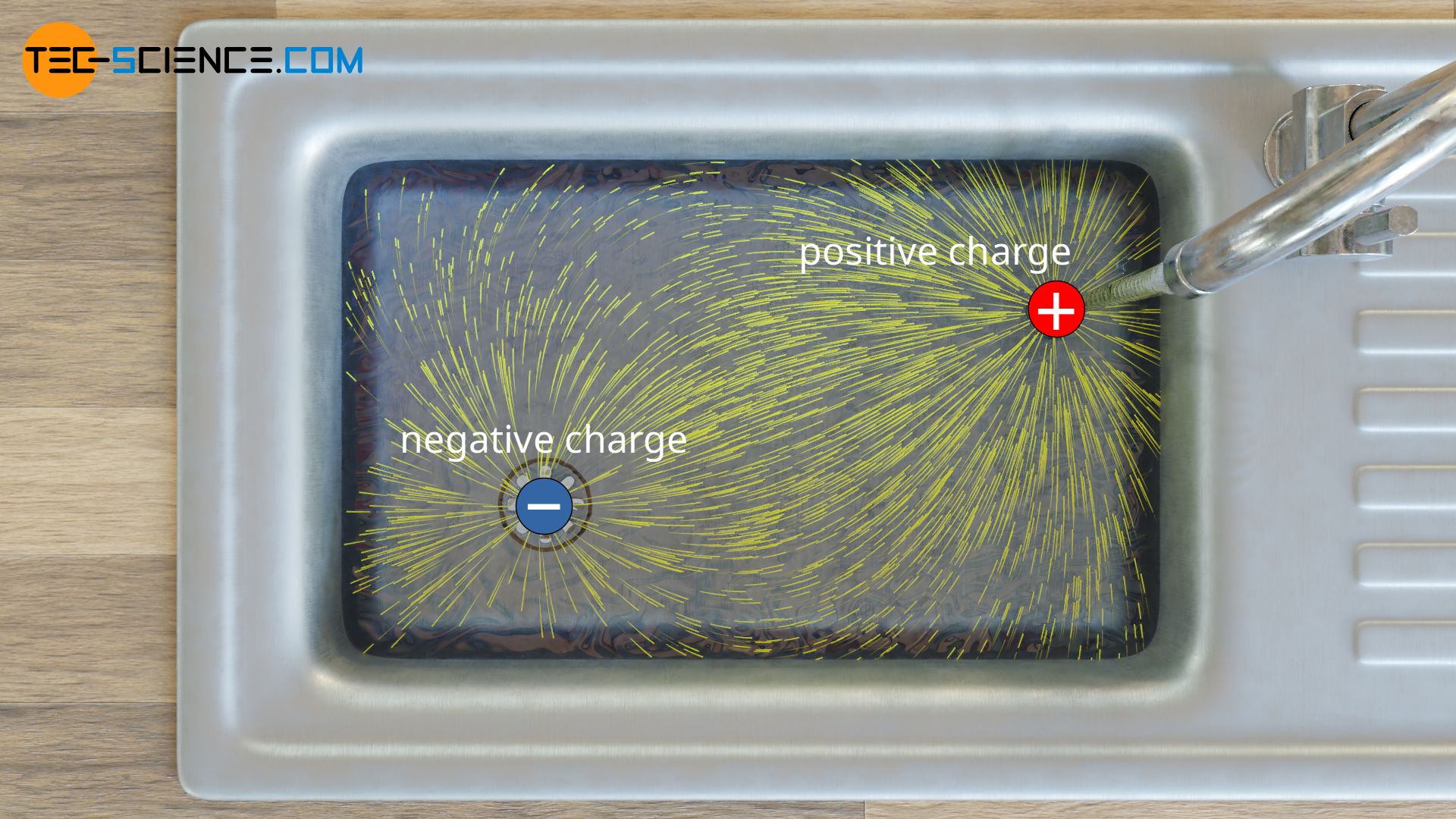
The figure below schematically shows a two-dimensional flow field. You can imagine pouring water into a sink and leaving the drain open at the same time. The resulting velocity field would then correspond in a simplified way to the flow field shown.

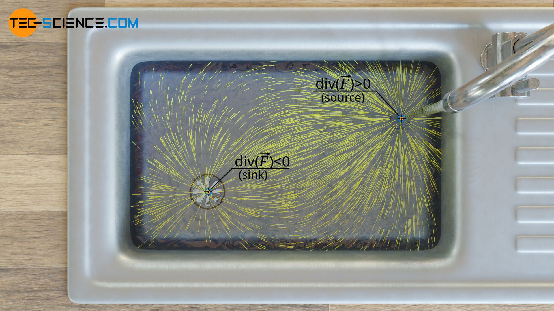
At the point where the water meets the sink, there is a water source. At this point the water is created in the flow plane, so to speak (note that we are looking at the two-dimensional case here and not the three-dimensional case, where obviously water cannot be created out of nothing). At the point where the drain is, the water disappears from a two-dimensional perspective. At this point, the water in the flow plane is annihilated, so to speak.

If you would apply the divergence operator to this vector field, you would get a positive value at the point where the water is created. At the point where the water is annihilated, you would get a negative value. By applying the divergence operator to a vector field, you can visualize the sources and sinks of vector fields in a vivid way. Field lines or flow lines start at points of positive divergence (sources) and end at points of negative divergence (sinks). The fact, that field lines or streamlines diverge strongly at sources or sinks, is finally the reason for the name of the operator.

The divergence operator converts a vector field into a scalar field, and the scalar quantities are a measure for the strength of a field source! Positive values indicate sources and negative values indicate sinks of field lines!

Instead of the flow field shown above you can also imagine two electric charges. The resulting field lines would look very similar. In fact, the divergence as a measure for the strength of a source (measure of the electric charge) plays a major role in this field, too. The divergence operator is therefore of great importance for many vector fields.

But there are also vector fields that have no sources or sinks and are therefore source-free. These include, for example, magnetic fields whose field lines have no beginning and no end, but are always closed. Even incompressible flows are obviously source-free due to the fact that mass cannot be created or annihilated (note: the above example of the 2D flow field only served as an illustrative example).