Derivation of the Bernoulli equation

The Bernoulli equation describes the relationship between static, dynamic and hydrostatic pressure for inviscid and incompressible fluids.

Static, dynamic and hydrostatic pressure

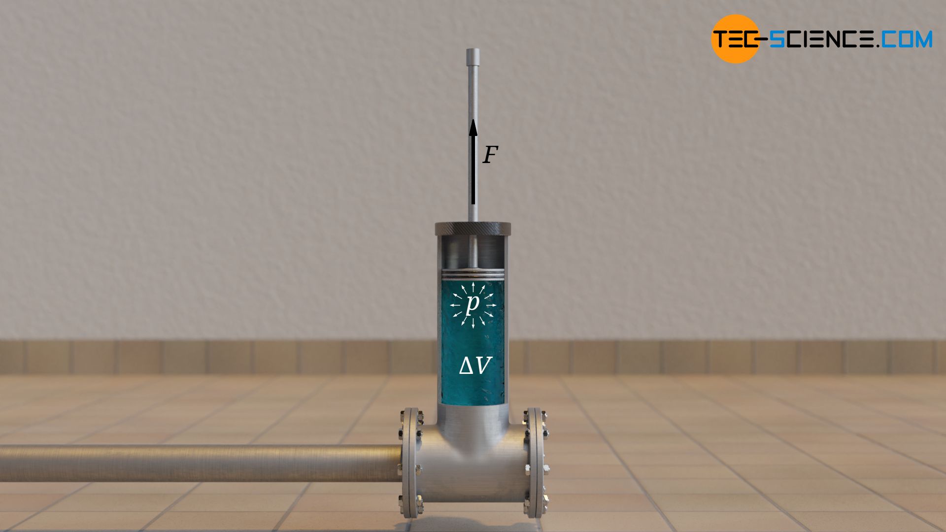
Due to the pressure acting in resting fluids, a force is exerted on interfaces. This force is able to do mechanical work, for example when the force acts on the piston in a cylinder. In the article Venturi effect it was already explained in detail that pressure can therefore be interpreted as a volume-specific energy. The pressure indicates how much potential energy per unit volume is present in a fluid and can be converted into mechanical work:

\begin{align}
\label{p}
& \boxed{p= \frac{\Delta W}{\Delta V}} \\[5px]
\end{align}

A resting fluid can only perform work based on static pressure, i.e. the pressure that arises due to the random microscopic motion of the molecules when they collide with an interface (see article Pressure in Gases). However, if a fluid flows (ordered macroscopic bulk motion), then the fluid can also perform work due to the kinetic energy associated with the motion. If this kinetic energy is related to the fluid volume, then the kinetic energy can also be assigned to a pressure according to equation (\ref{p}). In contrast to static pressure, in this case we speak of dynamic pressure. To put it simply:

The static pressure is connected with the random microscopic motion of the molecules, while the dynamic pressure is connected with the ordered macroscopic bulk motion of the flowing fluid!

Depending on the reference level, a fluid also has gravitational positional energy which can also be converted into work. This energy is used, for example, in hydroelectric power plants. According to the equation (\ref{p}), the potential energy contained per unit volume corresponds to a certain pressure. This pressure is called hydrostatic pressure!

If no energy is supplied to a flow from an external source, the sum of static energy (“pressure energy”), kinetic energy and gravitational potential energy must remain constant for reasons of energy conservation. For horizontal flows or for flows of fluids with low density (e.g. gases), changes in gravitational potential energies are not present or negligible. In these cases, an increase in kinetic energy thus inevitably means a decrease in static energy.

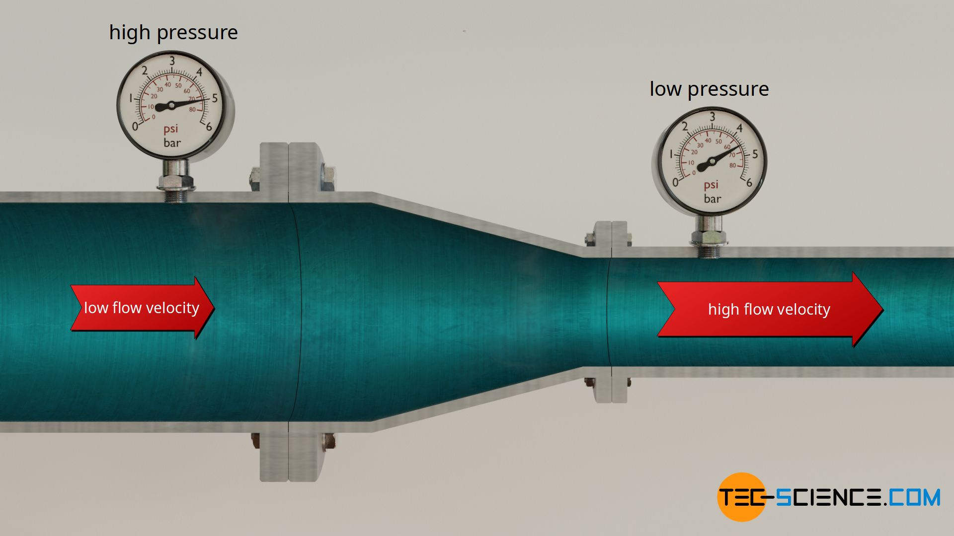
Such cases occur with horizontal pipes when the cross-section is reduced. Due to mass conservation, no mass can accumulate in the pipe or can be annihilated. The mass flow rate is therefore the same at every point along the pipe. In the case of smaller cross-sections, the flow velocity must therefore be greater so that the same mass can flow through per unit of time.

A decrease in cross-sectional area thus inevitably means an increase in flow speed. The resulting increase of kinetic energy can only come from static energy, as long as no energy is supplied (e.g. by a pump). Thus static pressure will decrease in favor of dynamic pressure. In the article Venturi effect, this phenomenon of decreasing pressure with increasing flow speed has already been discussed in detail.

As mentioned before, gravitational positional energies have to be taken into account when the fluid overcomes a certain height. The relationship between height, flow velocity and static pressure will be derived in the following.

Derivation of the Bernoulli equation

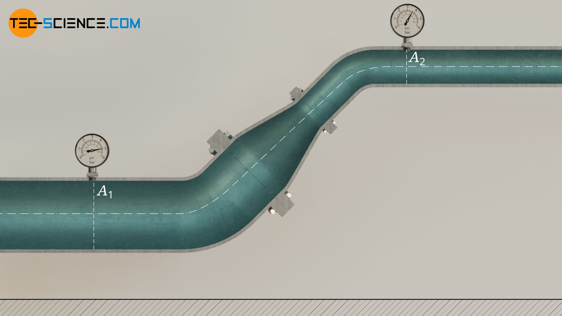
For the derivation of the relationship we consider a incompressible inviscid flow in a pipe without any friction. The pipe has a varying cross-section and overcomes a certain height.

Pressure energy (“pushed-in” and “pushed-out” energy)

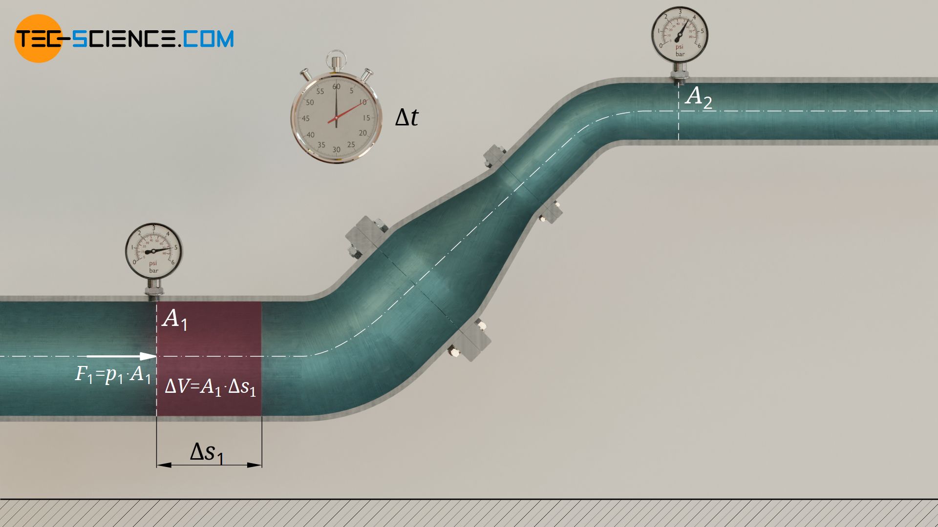
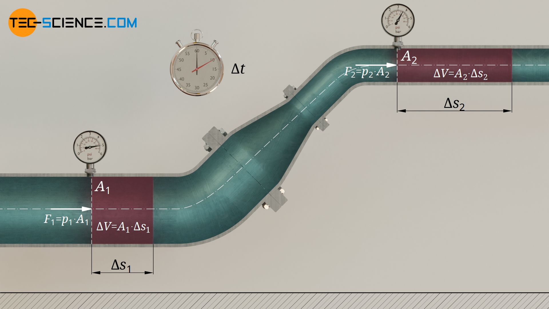
Let us first look at the lower part of the pipe section at point 1, where the static pressure p₁ acts. Within a certain time period Δt this pressure forces a certain fluid mass Δm through the pipe cross-section A₁. The distance by which the considered fluid element is pushed in, is denoted by Δs₁. The pressure energy W₁ with which the fluid element is pushed through the pipe at point 1 due to the static pressure (“pushed-in” energy) depends on the pushed-in fluid volume ΔV:

\begin{align}
& W_1 = F_1 \cdot \Delta s_1= p_1 \underbrace{A_1 \cdot \Delta s_1}_{\Delta V} \\[5px]
& \underline{W_1 = p_1 \Delta V} ~~~~~\text{“pushed-in” energy}\\[5px]
\end{align}

Now we look at the upper part of the pipe at point 2, where there is a lower static pressure p₂ due to the relationships explained in the previous section. However, within the considered time period Δt, the same fluid mass must be pushed through the reduced cross-section A₂ (conservation of mass). Since an incompressible fluid is assumed, the same fluid volume ΔV flows through A₂ as through A₁.

With the reduced cross-section A₂, however, this means a larger distance Δs₂ and thus a higher flow velocity! Due to the static pressure p₂ acting there, the fluid element is pushed through the pipe at point 2 with the following pressure energy W₂ (“pushed-out” energy):

\begin{align}
& W_2 = F_2 \cdot \Delta s_2= p_2 \underbrace{A_2 \cdot \Delta s_2}_{\Delta V} \\[5px]
& \underline{W_2 = p_2 \Delta V} ~~~~~\text{“pushed-out” energy}\\[5px]
\end{align}

Work required for accelerating and lifting the fluid

In practice one will notice that the pressure energy W₁ with which the fluid element was pushed into the pipe section at point 1 is greater than the pressure energy W₂ with which it is pushed out at point 2. The reason for this is that part of the “pushed-in” energy had to be used to accelerate the fluid element (supply of kinetic energy) and to lift the fluid against gravity (supply of gravitational potential energy). The “push-in” energy, minus the work required to accelerate and lift the fluid, gives the remaining “push-out” energy. In other words, the difference in pressure energy is the sum of acceleration work ΔW_a and lifting work ΔW_h:

\begin{align}
\label{a}
& \boxed{W_1 – W_2 = \Delta W_\text{a} + \Delta W_\text{h}} \\[5px]
\end{align}

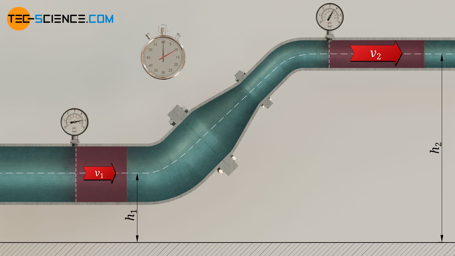
The work required to accelerate the fluid element from v₁ to v₂ is determined by difference in the kinetic energies at point 2 and point 1 (note: Δm=ϱ⋅ΔV):

\begin{align}
& \Delta W_\text{a} = W_\text{kin,2} -W_\text{kin,1} \\[5px]
& \underline{\Delta W_\text{a} = \frac{1}{2} \cdot \rho \Delta V \cdot v_2^2 ~- \frac{1}{2} \cdot \rho \Delta V \cdot v_1^2} \\[5px]
\end{align}

The work required to lift the fluid element from height h₁ to height h₂ is determined by difference in the gravitational potential energies at point 2 and point 1:

\begin{align}
& \Delta W_\text{h} = W_\text{h,2} – W_\text{h,1}\\[5px]
& \underline{\Delta W_\text{h} =\rho \Delta V \cdot g \cdot h_2 – \rho \Delta V \cdot g \cdot h_1}\\[5px]
\end{align}

Bernoulli equation

If the previous formulas are used in equation (\ref{a}), then the following relationship between the pressure energies, the kinetic energies and the gravitational potential energies at the two points under consideration can be deduced:

\begin{align}
\label{1}
& \underbrace{p_1 {\Delta V} – p_2 {\Delta V}}_{\text{pressure energies}} = \underbrace{\frac{1}{2} \rho {\Delta V} v_2^2 – \frac{1}{2} \rho {\Delta V} v_1^2}_{\text{kinetic energies}} + \underbrace{\rho {\Delta V} g h_2 – \rho {\Delta V}g h_1}_{\text{gravitational potential energies}} \\[5px]
\end{align}

All energy terms contain the fluid volume. This equation can therefore be divided by the fluid volume and is therefore independent of it:

\begin{align}
\label{2}
& p_1 – p_2 = \frac{1}{2} \rho v_2^2 – \frac{1}{2} \rho v_1^2 + \rho g h_2 – \rho g h_1 \\[5px]
\end{align}

Rearranging this equation finally results in the following relationship between two states 1 and 2 in a flow:

\begin{align}
& \boxed{p_1 + \frac{1}{2} \rho v_1^2 +\rho g h_1= p_2 + \frac{1}{2} \rho v_2^2 + \rho g h_2} ~~~\text{Bernoulli equation} \\[5px]
&\text{or}\\[5px]
& \boxed{p + \frac{1}{2} \rho ~v^2 +\rho g h= \text{constant}}=p_\text{tot} \\[5px]
\end{align}

This equation is also known as the Bernoulli equation. The terms found in the Bernoulli equation all have the dimension of a pressure. The term ½⋅ϱ⋅v², which is related to the kinetic energy of the fluid, is called hydrodynamic pressure or just dynamic pressure. The term ϱ⋅g⋅h, associated with the gravitational potential energy, is referred to as hydrostatic pressure. In contrast to these pressure terms, the pressure p is called static pressure.

pressure type	term	energetically linked with
static pressure	p	pressure energy (per unit fluid volume)
dynamic pressure	½⋅ϱ⋅v²	kinetic energy (per unit fluid volume)
hydrostatic pressure	ϱ⋅g⋅h	gravitational potential energy (per unit fluid volume)

In the article Exercises with solutions based on the Bernoulli equation, a few examples of the application of the Bernoulli equation are shown in more detail.

The Bernoulli equation states that the sum of static pressure, dynamic pressure and hydrostatic pressure is constant for a inviscid and incompressible fluid (as long as no energy is supplied from an external source, e.g. by a pump). The constant sum of these pressures is also called total pressure p_tot. For the application of the Bernoulli equation one can always imagine any fluid element moving along a streamline. The Bernoulli equation then links the states of two arbitrary points on this streamline.

The Bernoulli equation states that along a streamline the sum of static pressure, dynamic pressure and hydrostatic pressure is constant. In this form, it applies only to a friction-free (inviscid) and incompressible flow, without external energy supply.

Note that due to the viscosity of any fluids (internal friction), no flow is completely friction-free. In practice, this means energy dissipation and is associated with an additional (static) pressure loss. More on this later.

Important notes

It is important to understand that the Bernoulli equation is a (volume specific) energy equation. This is due to the step from equation (\ref{1}) to equation (\ref{2}), where the different forms of energy (pressure energy, kinetic energy and gravitational potential energy) were related to the fluid volume ΔV. The denotation as a pressure for the individual terms that occur in the Bernoulli equation is only of a formal nature, since each of them has the dimension of a pressure. However one should always keep in mind, that these pressures are based on energies.

Otherwise, the classical interpretation of pressure as “force per unit area” often leads to misunderstandings, especially with dynamic pressure. With this interpretation, it is very difficult to understand why static pressure decreases when the flow speed increases. It is often wrongly assumed that a high flow velocity means a large “force” and thus a high pressure.

When interpreted as energy, however, it becomes immediately clear that the increase in kinetic energy can only take place at the expense of pressure energy. Consequently, the static pressure will decrease with an increase in flow speed! This phenomenon is also called the Venturi effect and is explained in more detail in the linked article.

In fact, the term hydrostatic pressure is to be understood differently in this context than it is perhaps known from the hydrostatic pressure of a water column. In Bernoulli’s equation, hydrostatic pressure should not be interpreted as “force per unit area”. With regard to the Bernoulli equation, any hydrostatic pressure can be assigned to a point in a flow, depending on which reference level is chosen for the height. However, this does not of course change the forces acting in the fluid just because a different reference level is chosen.

In this case, the hydrostatic pressure is again to be interpreted as energy, i.e. as gravitational potential energy that is present per unit volume. This gravitational potential energy depends on the chosen reference level and therefore also the hydrostatic pressure defined by it.

Extended Bernoulli equation taking losses into account

Since pressure is a form of (volume-specific) energy, a loss of energy inevitably means a loss of pressure. Such a pressure loss occurs simply because every fluid has a certain viscosity. The fluid layers at the pipe wall adhere to it due to the so-called no-slip condition, and the layers further inside must therefore be displaced against each other if the fluid is to flow. This results in internal friction of the fluid, which ultimately means a loss of energy and thus a loss of pressure (see also Poiseuille flow).

Further energy losses occur in turbulent flows due to the turbulence. The roughness of the pipe wall plays a major role here. Flow losses and thus pressure losses also occur in components in a pipe system such as valves, pipe bends, reducers, etc. (more on this in the article Pressure loss in pipe systems).

The driving energy of a flow, given by the difference of the pushed-out energy W₂ and pushed-in energy W₁ between inlet and outlet of a considered flow section, must therefore not only accelerate and lift the flow against gravity, but also compensate for friction. Equation (\ref{a}) must therefore be extended by a energy loss term ΔW_loss:

\begin{align}
& \boxed{W_1 – W_2 = \Delta W_\text{b} + \Delta W_\text{h} + \Delta W_\text{loss}} \\[5px]
\end{align}

Equation (\ref{1}) thus has the general form:

\begin{align}
& \underbrace{p_1 {\Delta V} – p_2 {\Delta V}}_{\text{pressure energies}} = \underbrace{\frac{1}{2} \rho {\Delta V} v_2^2 – \frac{1}{2} \rho {\Delta V} v_1^2}_{\text{kinetic energies}} + \underbrace{\rho {\Delta V} g h_2 – \rho {\Delta V}g h_1}_{\text{gravitational potential energies}} + \underbrace{\Delta W_\text{loss}}_{\text{energy loss}}\\[5px]
\end{align}

Dividing this equation by the fluid volume ΔV provides the extended Bernoulli equation that takes into account energy losses:

\begin{align}
& \boxed{p_1 + \frac{1}{2} \rho v_1^2 +\rho g h_1= p_2 + \frac{1}{2} \rho v_2^2 + \rho g h_2 + \Delta p_\text{loss}}~~~\text{where}~~~\boxed{\Delta p_\text{loss} = \frac{\Delta W_\text{loss}}{\Delta V}} \\[5px]
\end{align}

The term W_loss/ΔV corresponds to the energy loss per unit volume and therefore represents to the pressure loss Δp_loss. Such a pressure loss is basically only noticeable in the static pressure, since the dynamic and hydrostatic pressures are predetermined by the flow velocities and heights. The static pressure p₂ downstream is reduced by this pressure loss:

\begin{align}
& p_2 = p_1 + \frac{1}{2} \rho \left(v_1^2-v_2^2\right) +\rho g (h_1-h_2) \color{red}{- \Delta p_\text{loss}} \\[5px]
\end{align}