Derivation of the Euler equation of motion (conservation of momentum)

The Euler equation of motion describes inviscid, unsteady flows of compressible or incompressible fluids.

Pressure forces on a fluid element

The Euler equation is based on Newton’s second law, which relates the change in velocity of a fluid particle to the presence of a force. Associated with this is the conservation of momentum, so that the Euler equation can also be regarded as a consequence of the conservation of momentum.

For the derivation of the Euler equation we consider an infinitesimal fluid volume dV with mass dm. We describe the motion of the fluid element from a fixed coordinate system (so-called Eulerian approach). By definition, the considered fluid element moves along an arbitrarily oriented streamline.

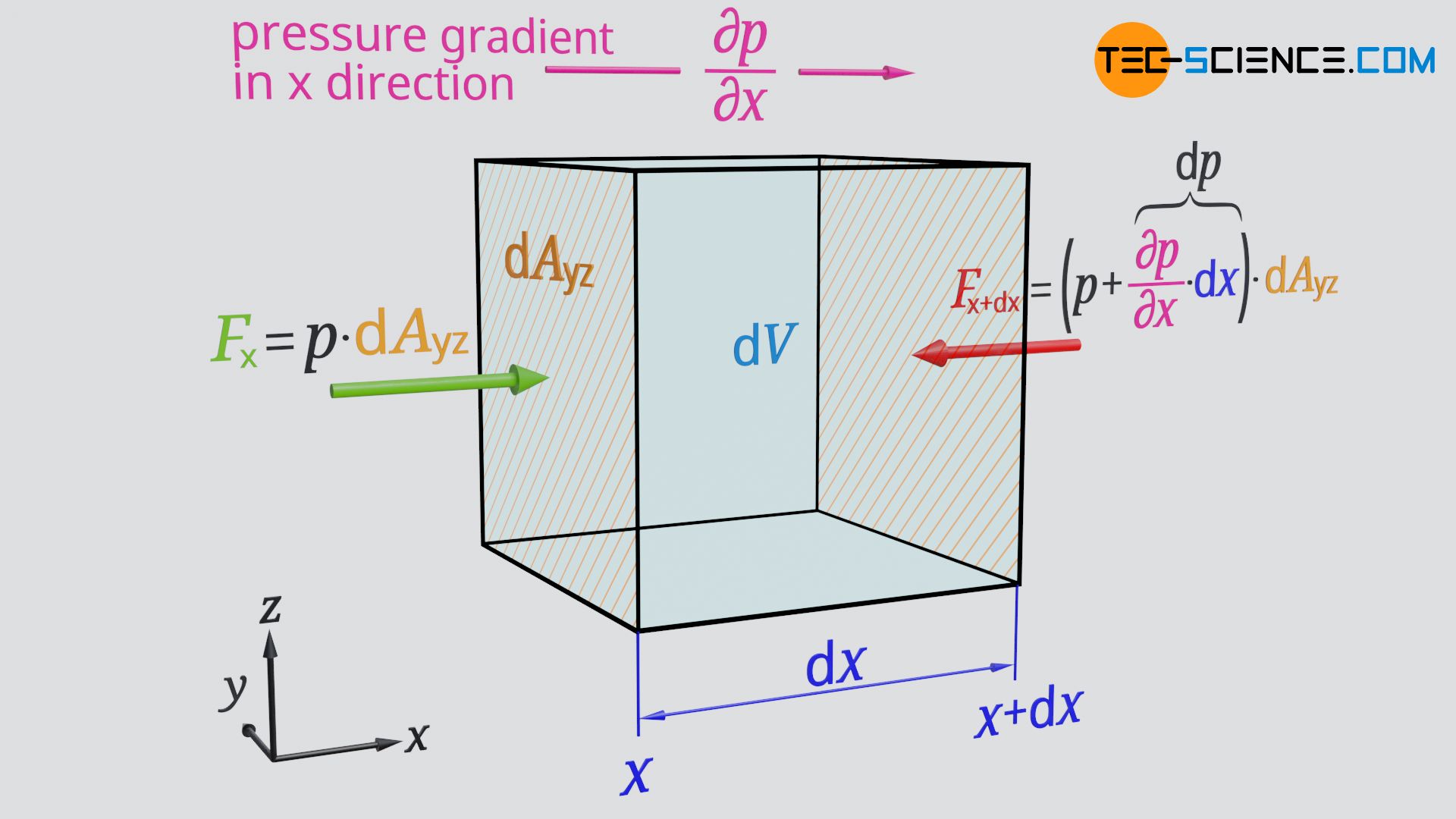
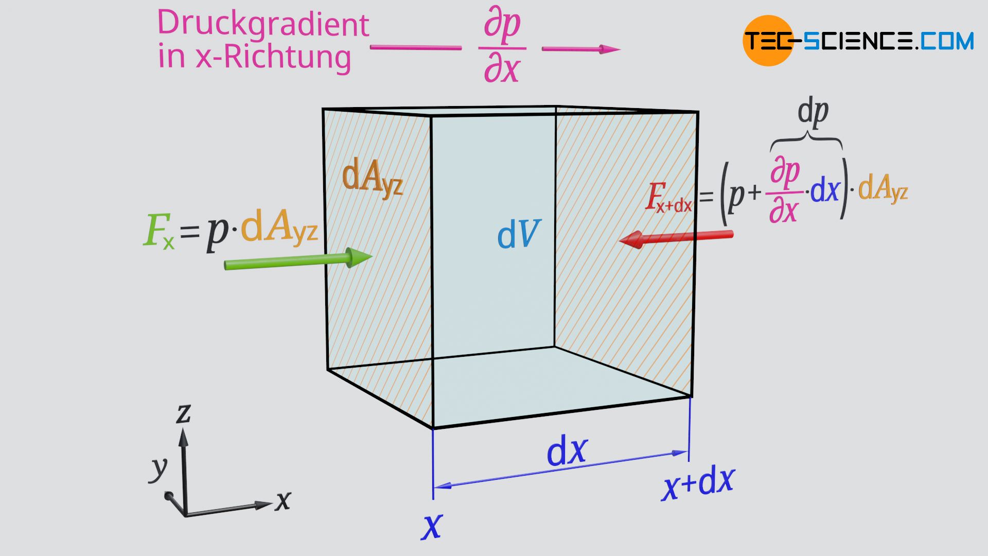
First we consider the motion of the fluid element only in x-direction. At a position x a pressure p is present. At this location the force F_x acts on the surface dA_yz of the fluid element:

\begin{align}
&\underline{F_\text{x} = p \cdot \text{d}A_\text{yz}} \\[5px]
\end{align}

The pressure is not constant in a flow, but changes locally. This is because pressure differences are ultimately the reason why a flow comes about at all. Therefore, the pressure in the x-direction will change. For a given pressure gradient ∂p/∂x (which can be positive or negative!), the following pressure change dp_x results over the length dx of the fluid element:

\begin{align}
&\underline{\text{d}p_\text{x} =\frac{\partial p}{\partial x} \cdot \text{d}x} ~~~~~\text{pressure change along }\text{d}x \\[5px]
\end{align}

This pressure change leads to the following force F_x+dx at the position x+dx:

\begin{align}
&F_{\text{x+d}x}= \left(p + \text{d}p_\text{x} \right) \cdot \text{d}A_\text{yz} \\[5px]
&\underline{F_{\text{x+d}x} = \left(p + \frac{\partial p}{\partial x} \cdot \text{d}x \right) \cdot \text{d}A_\text{yz}} \\[5px]
\end{align}

The forces F_x and F_x+dx acting on the surfaces dA_yz are in opposite directions, so that the following resultant pressure force F_px acts in x-direction, which causes/influences the motion of the fluid element in x-direction:

\begin{align}
\require{cancel}
&F_\text{px} = F_\text{x} – F_{\text{x+d}x} \\[5px]
&F_\text{px} = p \cdot \text{d}A_\text{yz} – \left(p + \frac{\partial p}{\partial x} \cdot \text{d}x \right) \cdot \text{d}A_\text{yz} \\[5px]
&F_\text{px} = \cancel{p \cdot \text{d}A_\text{yz}} – \cancel{p \cdot \text{d}A_\text{yz}} – \frac{\partial p}{\partial x} \cdot \underbrace{\text{d}x \cdot \text{d}A_\text{yz}}_{\text{d}V} \\[5px]
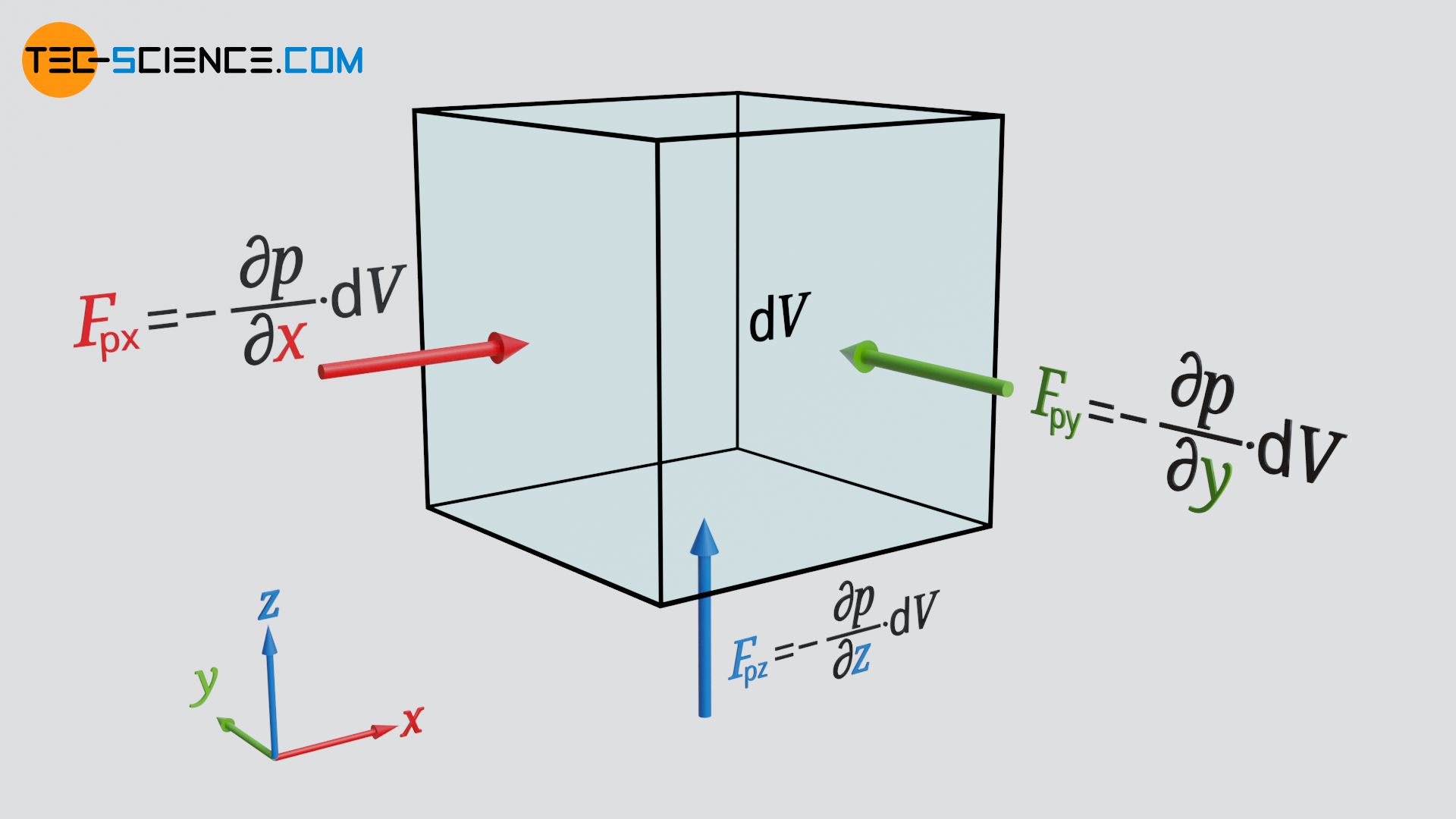
&\boxed{F_\text{px} = – \frac{\partial p}{\partial x} \cdot \text{d}V} ~~~~~\text{pressure force in x direction} \\[5px]
\end{align}

The negative sign indicates that with a positive pressure gradient ∂p/∂x>0 the force on the fluid element is directed against the positive x-direction, since the pressure obviously increases along the fluid element. The fluid element would thus be slowed down in the x direction if it were to move in positive x direction. The same considerations we have made for the x direction can be made for the y and z directions. This leads to the following equations:

\begin{align}
&\boxed{F_\text{py} = – \frac{\partial p}{\partial y} \cdot \text{d}V}~~~~~\text{pressure force in y direction} \\[5px]
&\boxed{F_\text{pz} = – \frac{\partial p}{\partial z} \cdot \text{d}V}~~~~~\text{pressure force in z direction} \\[5px]
\end{align}

In these equations, ∂p/∂y and ∂p/∂z indicate the pressure gradients in y and z direction, respectively.

Vector notation of the pressure force

The pressure forces F_px, F_py and F_pz calculated on the basis of the respective gradients can be written line by line as a vector F_p for the pressure force:

\begin{align}
&\vec{F_\text{p}} = \begin{pmatrix}F_\text{px} \\\ F_\text{py} \\\ F_\text{pz} \end{pmatrix} = \begin{pmatrix}-\frac{\partial p}{\partial x}\cdot \text{d}V \\\ -\frac{\partial p}{\partial y}\cdot \text{d}V \\\ -\frac{\partial p}{\partial z} \cdot \text{d}V \end{pmatrix} = -\begin{pmatrix}\large\frac{\partial p}{\partial x} \\\ \large\frac{\partial p}{\partial y} \\\ \large\frac{\partial p}{\partial z} \end{pmatrix} \cdot \text{d}V\\[5px]
\end{align}

The term in brackets corresponds to the pressure gradient and can be expressed by the del operator, denoted by the nabla symbol ∇ (often the arrow above the symbol is not shown; formally, however, the del operator is a vector!)

\begin{align}
&\boxed{\vec F_\text{p} =- \vec \nabla p \cdot \text{d}V } ~~~\text{mit:}~~~\boxed{\vec \nabla =\begin{pmatrix}\large\frac{\partial}{\partial x}\\\ \large\frac{\partial }{\partial y} \\\ \large\frac{\partial}{\partial z} \end{pmatrix}} ~~~\text{del operator}\\[5px]
& \vec \nabla p = \text{pressure gradient} \\[5px]
\end{align}

Note that applying the del operator to a scalar field (here: spatial pressure distribution) results in a vector field. The vectors point in the direction of the greatest increase of the scalar quantity (here: in the direction of the greatest pressure increase).

It should again be noted that the negative sign in the formula above indicates that the pressure force F_p acting on a fluid volume dV is directed against the pressure gradient ∇p. A fluid element is thus accelerated in the direction of decreasing pressure, provided that no further forces act on the fluid element.

Shear forces and field forces

In a flow, the velocity is generally neither constant in time nor in space. Thus, the fluid flows either slower or faster past the lateral surfaces of the considered fluid element. Therefore internal frictional forces occur, which are the greater the more viscous the fluid is. However, since we assume a friction-free flow and thus a inviscid fluid, such shear forces do not occur in the flow.

Other forces that act on the fluid element but cannot be neglected in general are field forces such as those caused by gravity. For example, air flow on earth or flows in pipes are significantly influenced by gravity. For example, in flows containing ferromagnetic fluid particles, an external magnetic field also influences the flow.

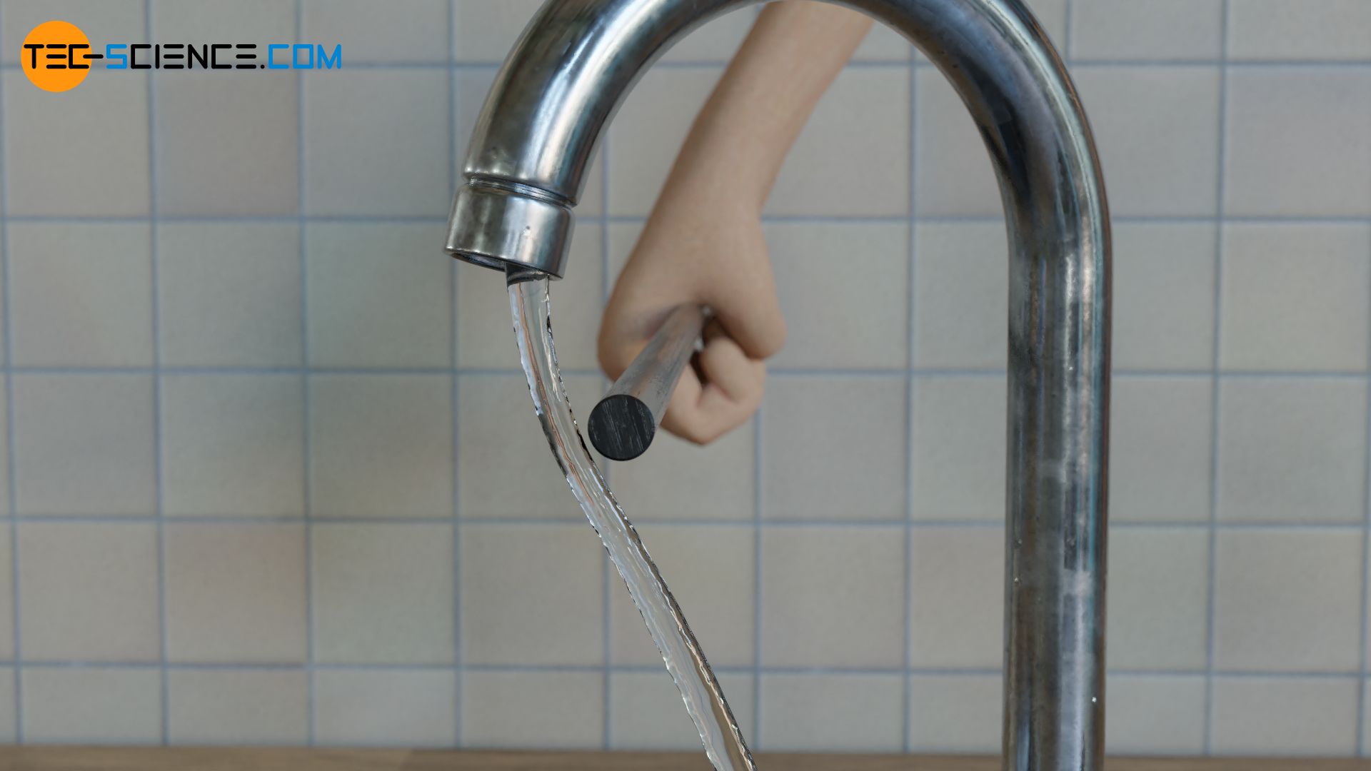
Also electrically charged particles in a fluid are possible, so that the flow is then influenced by an external electric field. Water is already influenced by the dipole interaction of the H₂O molecules in an electric field without the need to contain electrically charged particles. This can be demonstrated with an electrically charged plastic rod. If the charged plastic rod is brought into the vicinity of a thin water jet, it is observed that the jet is deflected.

Thus, a fluid element is affected not only by the pressure force F_p, but also by field forces F_g (the weight force should only be representative of other possible field forces!) The sum of both forces then corresponds to the accelerating force F_a (resultant force), which influences the motion of the fluid element:

\begin{align}
& \vec{F}_\text{a} = \vec F_\text{g}+ \vec F_\text{p}\\[5px]
\label{besch}
&\boxed{\vec{F}_\text{a} = \vec F_\text{g}- \vec \nabla p \cdot \text{d}V } ~~~~~\text{accelerating force on a fluid element}\\[5px]
\end{align}

Newton’s second law (substantial acceleration)

According to Newton’s second law, the accelerating force F_a leads to a change in velocity (acceleration), which depends on the mass dm of the fluid element. This material acceleration is also called substantial acceleration a_sub:

\begin{align}
& \boxed{\vec a_\text{sub} = \frac{\vec F_\text{a}}{\text{d}m}} ~~~~~\text{Newton’s second law}\\[5px]
& \vec a_\text{sub} = \frac{\vec F_\text{g}- \vec \nabla p \cdot \text{d}V}{\text{d}m} \\[5px]
& \vec a_\text{sub} = \frac{\vec F_\text{g}}{\text{d}m}- \frac{\vec \nabla p \cdot \text{d}V}{\text{d}m}
~~~\text{where} ~~~\text{d}m=\rho \cdot \text{d}V ~~~\text{:}\\[5px]
& \vec a_\text{sub} = \underbrace{\frac{\vec F_\text{g}}{\text{d}m}}_{\text{specific field force } g}- \frac{\vec \nabla p \cdot \text{d}V}{\rho \cdot \text{d}V} \\[5px]
\label{eu}
& \boxed{\vec a_\text{sub} = \vec g- \frac{1}{\rho} \vec \nabla p} ~~~~~\text{substantial acceleration}\\[5px]
\end{align}

The quotient of field force F_g and mass dm can generally be interpreted as field force per unit mass. In the case of gravity this quotient corresponds to the gravitational acceleration g. If other field forces such as magnetic or electrical forces are also involved, these must also be taken into account in the equation as mass-specific field forces.

Temporal and convective acceleration

The substantial acceleration, i.e. the actually observable acceleration of a fluid element, can be traced back to two causes. On the one hand, a flow and thus the velocity of a fluid element changes not only in time but also in place. Substantial acceleration is thus attributed to a temporal component (temporal acceleration) and a local component (convective acceleration).

We can imagine an air flow on a windy day. The wind blows with a constantly changing direction (unsteady flow). We observe the situation how the wind blows around the corner of a house. A fluid element viewed at a certain location changes its velocity from one second to the next. This is a consequence of the permanently changing flow over time. The resulting acceleration is therefore also called temporal acceleration or local acceleration a_loc, because it is a consequence of the changing velocity at a fixed location.

One could now conclude that in a steady flow, where the speed does not change in time, there is no acceleration on the fluid particles. However, this is not the case. Although the speed of a stationary flow does not change in time at a fixed location, a fluid particle generally has to change its velocity permanently while flowing. For example, the speed of a pipe flow is greater at a constricted section compared to a point at a larger cross-section. Thus, a fluid particle is generally still accelerated when it changes location, despite the lack of temporal change in the flow.

Even the steady flow of wind around a corner constantly requires the fluid particle to adapt to the new flow direction and thus to accelerate. The acceleration due to the change of location is therefore also called convective acceleration a_con.

In summary, it can be concluded that

• The temporal or local acceleration is due to the time-varying flow velocity of an unsteady flow at a fixed location.
• The convective acceleration is due to the flow velocity changing from place to place.
• Both acceleration components together result in the observable acceleration, which is also called substantial or material acceleration.

Note that there is no local acceleration in a steady flow, because the flow velocity does not change in time!

Relationship between local, convective and substantial acceleration

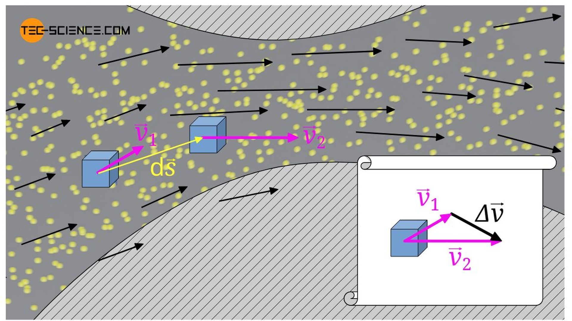
For the sake of simplicity, we first look at a fluid particle on a streamline s and we describe the motion on this streamline (one-dimensional motion). The substantial change in velocity dv, i.e. the actually observable change in velocity, is obtained in this case from the temporal change of velocity ∂v/∂t within the time dt (temporal component) and from a spatial change of velocity ∂v/∂s (gradient) within the distance ds (convective component):

\begin{align}
&\underbrace{\text{d}v}_{\text{substantial change}} = \underbrace{\frac{\partial v}{\partial t} \text{d}t}_{\text{temporal change}} + \underbrace{\frac{\partial v}{\partial s} \text{d} s}_{\text{convective change}}\\[5px]
\end{align}

If this equation is divided by the time duration dt, the following formula for the substantial acceleration a_sub in tangential direction of the streamline is obtained:

\begin{align}
\require{cancel}
&\boxed{a_\text{sub} = \frac{\text{d}v}{\text{d}t}} = \frac{\partial v}{\partial t} \frac{\cancel{\text{d}t}}{\cancel{\text{d}t}}+ \frac{\partial v}{\partial s} \underbrace{\frac{\text{d}s}{\text{d}t}}_{v} \\[5px]
&a_\text{sub} = \underbrace{~~~~~\frac{\partial v}{\partial t}~~~~~}_{\text{local acceleration}} + \underbrace{~~~~~\frac{\partial v}{\partial s}v~~~~~}_{\text{convective acceleration}} \\[5px]
\end{align}

\begin{align}
& \boxed{a_\text{sub} = \frac{\partial v}{\partial t} + \frac{\partial v}{\partial s}v} &&\text{substantial acceleration}\\[5px]
& \boxed{a_\text{loc}=\frac{\partial v}{\partial t}} &&\text{local acceleration} \\[5px]
& \boxed{a_\text{con}= \frac{\partial v}{\partial s}v} &&\text{convective acceleration} \\[5px]
\end{align}

The term of convective acceleration obviously depends on the flow velocity. This becomes clear, because if the fluid element flows very fast, it covers a relatively large distance within a certain time. For a given velocity gradient ∂c/∂s this means a large change in velocity and thus a large acceleration.

Vector notation of the substantial acceleration

For the sake of simplicity, we have only considered the one-dimensional motion of a fluid particle on a streamline. In the three-dimensional case, i.e. when describing the motion from a fixed coordinate system, the local acceleration can also still be written relatively easily in vector notation:

\begin{align}
& \boxed{\vec a_\text{loc}=\frac{\partial \vec v}{\partial t} = \begin{pmatrix}\Large\frac{\partial v_x}{\partial t} \\\ \Large\frac{\partial v_y}{\partial t} \\\ \Large\frac{\partial v_z}{\partial t} \end{pmatrix} } ~~~~~\text{local acceleration} \\[5px]
\end{align}

In contrast to the local acceleration, the vector notation of the convective acceleration is much more complicated, since it is a location-dependency in three dimensions. Each velocity component changes not only due to a local change in one dimension, but is the consequence of a change in all three dimensions!

The velocity component in x direction will generally not only change when a fluid particle moves in x direction. For example, the velocity in x direction will also change if the fluid particle moves in y direction, because the flow velocity in x direction is lower there. A change of location in z direction also generally results in a change of velocity in the x direction, because the flow velocity in the x direction is higher there, for example.

The component of the convective acceleration in x direction (a_con,x) is thus due to the change of location in all three dimensions:

\begin{align}
& \underline{a_\text{con,x}=\frac{\partial v_\text{x}}{\partial x}v_\text{x} + \frac{\partial v_\text{x}}{\partial y}v_\text{y} + \frac{\partial v_\text{x}}{\partial z}v_\text{z}} ~~~~~\text{convective acceleration in }x\text{ direction} \\[5px]
\end{align}

Just for clarification: The velocity of a fluid particle in x direction will generally not only change when the position of the particle changes in x direction (velocity gradient ∂v_x/∂x), but also in case of a change of location in y direction (velocity gradient ∂v_x/∂y) or z direction (velocity gradient ∂v_x/∂z).

For the components of the convective acceleration in y- and z-direction the analogous considerations apply:

\begin{align}
& \underline{a_\text{con,y}=\frac{\partial v_\text{y}}{\partial x}v_\text{x} + \frac{\partial v_\text{y}}{\partial y}v_\text{y} + \frac{\partial v_\text{y}}{\partial z}v_\text{z}} ~~~~~\text{convective acceleration in }y\text{ direction} \\[5px]
& \underline{a_\text{con,y}=\frac{\partial v_\text{z}}{\partial x}v_\text{x} + \frac{\partial v_\text{z}}{\partial y}v_\text{y} + \frac{\partial v_\text{z}}{\partial z}v_\text{z}} ~~~~~\text{convective acceleration in }z\text{ direction} \\[5px]
\end{align}

Thus, the vector of the convective acceleration a_con is represented by 9 terms:

\begin{align}
& \boxed{\vec a_\text{con}= \large \begin{pmatrix} a_\text{con,x}\\\ a_\text{con,y}\\\ a_\text{con,z} \end{pmatrix} 
= \Large \begin{pmatrix}
\frac{\partial v_\text{x}}{\partial x}v_\text{x} + \frac{\partial v_\text{x}}{\partial y}v_\text{y} + \frac{\partial v_\text{x}}{\partial z}v_\text{z}
\\\
\frac{\partial v_\text{y}}{\partial x}v_\text{x} + \frac{\partial v_\text{y}}{\partial y}v_\text{y} + \frac{\partial v_\text{y}}{\partial z}v_\text{z}
\\\
\frac{\partial v_\text{z}}{\partial x}v_\text{x} + \frac{\partial v_\text{z}}{\partial y}v_\text{y} + \frac{\partial v_\text{z}}{\partial z}v_\text{z}
\end{pmatrix} 
} \\[0px]
\end{align}

The convective acceleration can be represented much more clearly using the del operator ∇:

\begin{align}
& \boxed{\vec a_\text{con} = \left(\vec v \cdot \vec \nabla \right) \vec v}~~~\text{convective acceleration} \\[5px]
\end{align}

For the vector of the substantial acceleration a_sub, as the sum of local and convective acceleration, thus the following formula applies:

\begin{align}
\label{en}
&\boxed{\vec a_\text{sub} = \frac{\partial \vec v}{\partial t} + \left(\vec v \cdot \vec \nabla \right) \vec v} ~\text{substantial acceleration} \\[5px]
& \boxed{\vec a_\text{sub}
= \Large \begin{pmatrix}
\frac{\partial v_x}{\partial t} + \frac{\partial v_\text{x}}{\partial x}v_\text{x} + \frac{\partial v_\text{x}}{\partial y}v_\text{y} + \frac{\partial v_\text{x}}{\partial z}v_\text{z}
\\\
\frac{\partial v_y}{\partial t} + \frac{\partial v_\text{y}}{\partial x}v_\text{x} + \frac{\partial v_\text{y}}{\partial y}v_\text{y} + \frac{\partial v_\text{y}}{\partial z}v_\text{z}
\\\
\frac{\partial v_z}{\partial t} + \frac{\partial v_\text{z}}{\partial x}v_\text{x} + \frac{\partial v_\text{z}}{\partial y}v_\text{y} + \frac{\partial v_\text{z}}{\partial z}v_\text{z}
\end{pmatrix} \\[5px]
}
\end{align}

Using equation (\ref{en}) in equation (\ref{eu}), one finally obtains the equation of motion of a fluid particle in a frictionless, unsteady flow. This equation is also known as the Euler equation of motion and applies to both incompressible and compressible fluids (as long as they are inviscid):

\begin{align}
& \vec a_\text{sub} = \vec g- \frac{1}{\rho} \vec \nabla p \\[5px]
&\frac{\partial \vec v}{\partial t} + \left(\vec v \cdot \vec \nabla \right) \vec v = \vec g- \frac{1}{\rho} \vec \nabla p \\[5px]
&\boxed{\frac{\partial \vec v}{\partial t} + \left(\vec v \cdot \vec \nabla \right) \vec v + \frac{1}{\rho} \vec \nabla p = \vec g}~~~\text{Euler equation of motion} \\[5px]
\end{align}

The Euler equation can also be given in components:

\begin{align}
& \boxed{\frac{\partial v_\text{x}}{\partial t} + \frac{\partial v_\text{x}}{\partial x}v_\text{x} + \frac{\partial v_\text{x}}{\partial y}v_\text{y} + \frac{\partial v_\text{x}}{\partial z}v_\text{z} + \frac{1}{\rho} \frac{\partial p}{\partial x} = g_\text{x}}~~~\text{Euler eq. in x-direction} \\[5px]
& \boxed{\frac{\partial v_\text{y}}{\partial t} + \frac{\partial v_\text{y}}{\partial x}v_\text{x} + \frac{\partial v_\text{y}}{\partial y}v_\text{y} + \frac{\partial v_\text{y}}{\partial z}v_\text{z} + \frac{1}{\rho} \frac{\partial p}{\partial y} = g_\text{y}}~~~\text{Euler eq. in y-direction} \\[5px]
& \boxed{\frac{\partial v_\text{z}}{\partial t} + \frac{\partial v_\text{z}}{\partial x}v_\text{x} + \frac{\partial v_\text{z}}{\partial y}v_\text{y} + \frac{\partial v_\text{z}}{\partial z}v_\text{z} + \frac{1}{\rho} \frac{\partial p}{\partial z} = g_\text{z}}~~~\text{Euler eq. in z-direction} \\[5px]
\end{align}

Note the following procedure when calculating convective acceleration using the Nabla operator:

\begin{align}
\vec a_\text{con} &= \left(\vec v \cdot \vec \nabla \right) \vec v\\[5px]
&= \left[\begin{pmatrix} v_x \\\ v_y \\\ v_z \end{pmatrix}
\cdot \begin{pmatrix} \frac{\partial}{\partial x} \\\ \frac{\partial}{\partial y} \\\ \frac{\partial}{\partial z} \end{pmatrix} \right] \cdot \begin{pmatrix} v_x \\\ v_y \\\ v_z \end{pmatrix}\\[5px]
&=\left[ v_x \frac{\partial}{\partial x} + v_y \frac{\partial}{\partial y} + v_z \frac{\partial}{\partial z} \right] \cdot \begin{pmatrix} v_x \\\ v_y \\\ v_z \end{pmatrix}\\[5px]
&=\Large \begin{pmatrix}
v_\text{x} \frac{\partial v_\text{x}}{\partial x} + v_\text{y} \frac{\partial v_\text{x}}{\partial y} +v_\text{z} \frac{\partial v_\text{x}}{\partial z}
\\\
v_\text{x} \frac{\partial v_\text{y}}{\partial x} + v_\text{y} \frac{\partial v_\text{y}}{\partial y} +v_\text{z} \frac{\partial v_\text{y}}{\partial z}
\\\
v_\text{x} \frac{\partial v_\text{z}}{\partial x} +v_\text{y} \frac{\partial v_\text{z}}{\partial y} +v_\text{z} \frac{\partial v_\text{z}}{\partial z}
\end{pmatrix} 
\end{align}

Using the Euler equation along a streamline (Bernoulli equation)

We would like to apply the Euler equation to a streamline and describe the change of state of a flow along this streamline. In this case we are dealing with a flow in only one dimension: in direction of the streamline. The locally changing velocity and pressure are denoted by v and p respectively. With s as the coordinate along the streamline, the Euler equation is as follows:

\begin{align}
&\frac{\partial v}{\partial t} + \frac{\partial v}{\partial s}v + \frac{1}{\rho} \frac{\partial p}{\partial s} = – g \cdot \cos(\alpha) \\[5px]
\end{align}

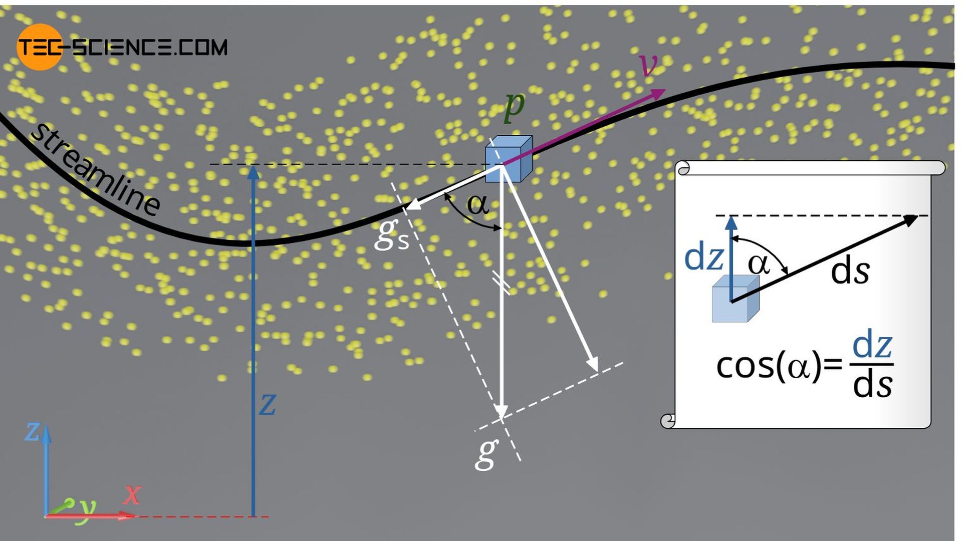
The angle α is the angle between the vertical z direction and the tangent of the streamline s. The term -g⋅cos(α) thus describes the component of the gravitational acceleration acting against the streamline, which leads to a decelerating force of the fluid particle at a positive angle α (hence the negative sign). An infinitesimal change on the streamline ds is related by the angle α to the infinitesimal change dz in z direction as follows:

\begin{align}
&\cos(\alpha) = \frac{\text{d}z}{\text{d}s}\\[5px]
\end{align}

Therefore the Euler equation of motion along the streamline is:

\begin{align}
&\frac{\partial v}{\partial t} + \frac{\partial v}{\partial s}v + \frac{1}{\rho} \frac{\partial p}{\partial s} = – g \frac{\text{d}z}{\text{d}s}\\[5px]
\end{align}

For the sake of simplicity, we assume in the following that the flow is steady and incompressible. In this case the velocity is not a function of time and thus the partial derivative of the velocity with respect to time is zero (∂v/∂t=0). Due to the incompressibility, the density is not a function of the location either. Instead of the partial derivatives with respect to the location, we can now write the total derivatives. We then get the following relationship between the infinitesimal changes of pressure, velocity and height along the streamline:

\begin{align}
\require{cancel}
&\cancel{\frac{\partial v}{\partial t}} + \frac{\text{d}v}{\text{d}s}v + \frac{1}{\rho} \frac{\text{d}p}{\text{d}s} = -g \frac{\text{d}z}{\text{d}s}\\[5px]
&\frac{\text{d} v}{\text{d}s}v + \frac{1}{\rho} \frac{\text{d}p}{\text{d}s} = -g \frac{\text{d}z}{\text{d}s}&&|\cdot \text{d}s\\[5px]
&v~\text{d}v + \frac{1}{\rho} \text{d}p = -g \text{d}z&&|\cdot \rho\\[5px]
&\underline{\text{d}p + \rho v ~\text{d}v ~ + \rho g ~\text{d}z = 0}\\[5px]
\end{align}

This equation describes the relationship between the infinitesimal changes in pressure, velocity and height along a streamline. We can now integrate this equation to obtain the relationships between the quantities themselves rather than the relationships between the changes in the quantities. The density and acceleration due to gravity, which are considered constant, can be written before the integral sign.

\begin{align}
&\int \left(\text{d}p + \rho v ~\text{d}v ~ + \rho g ~ \text{d}z \right)= \text{konstant}\\[5px]
&\int \text{d}p + \rho \int v ~\text{d}v ~ + \rho g ~\int \text{d}z = \text{konstant}\\[5px]
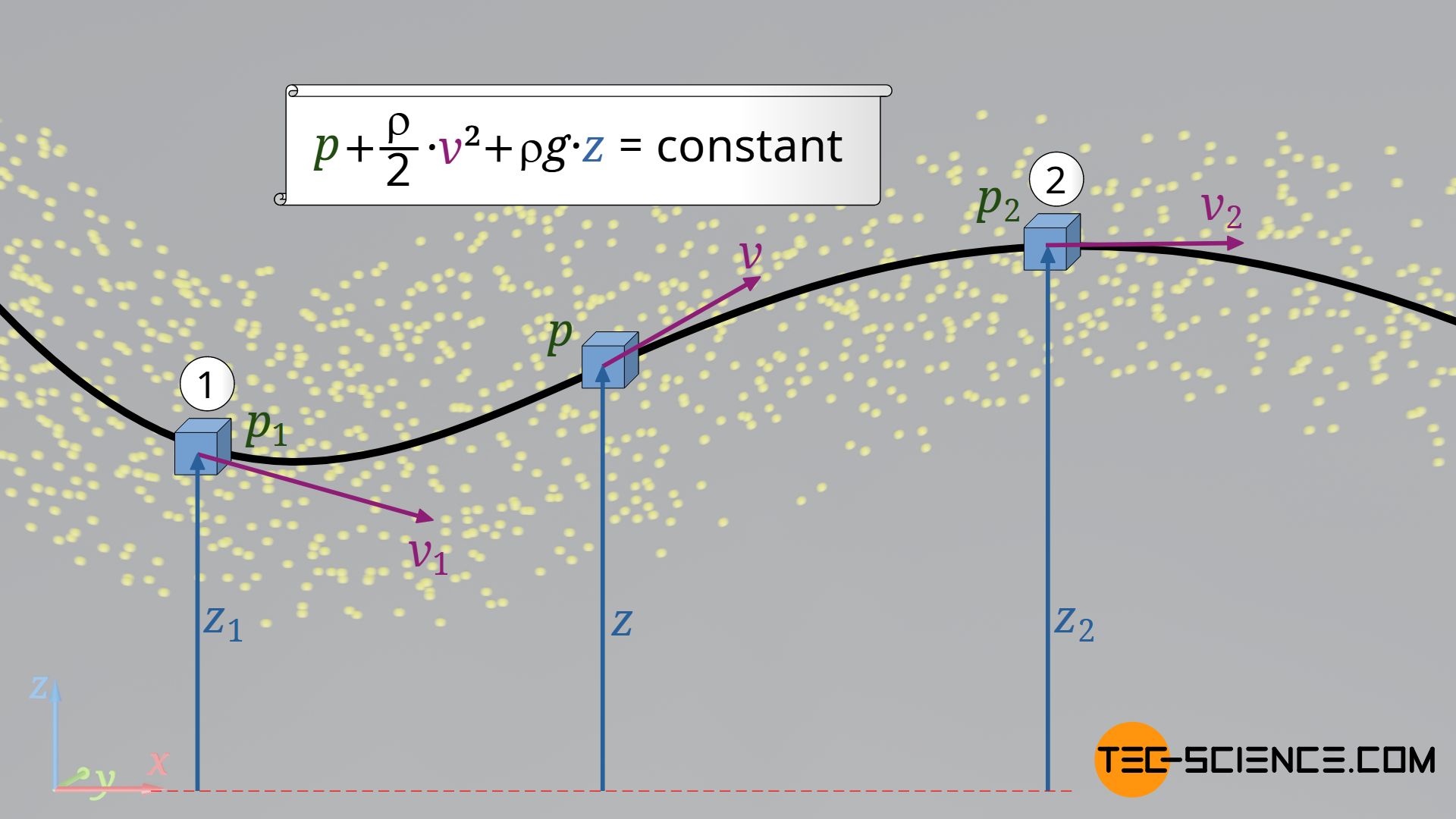
&\boxed{p + \frac{\rho}{2} v^2 + \rho g ~z = \text{konstant}}~~~\text{Bernoulli’s equation}\\[5px]
\end{align}

We finally obtain the Bernoulli equation for incompressible and frictionless fluids! This equation states that the sum of pressure energy, kinetic energy and positional energy along the streamline is constant (conservation of energy). Note that this equation is only valid for frictionless flows, i.e. especially for inviscid fluids. Two points on a streamline are thus linked in this friction-free case as follows:

\begin{align}
&\boxed{p_1 + \frac{\rho}{2} v_1^2 + \rho g ~z_1 =p_2 + \frac{\rho}{2} v_2^2 + \rho g ~z_2}\\[5px]
\end{align}

Exercises with solutions based on the Bernoulli equation can be found in the linked article.