Pressure losses in pipes are caused by internal friction of the fluid (viscosity) and friction between fluid and wall. Pressure losses also occur in components.
Introduction
When fluids flow through pipes, energy losses inevitably occur. On the one hand, this is due to friction that occurs between the pipe wall and the fluid (wall friction). On the other hand, frictional effects also occur within the fluid due to the viscosity of the fluid (internal friction). The faster the fluid flows, the greater the internal friction effect (see also the article on Poiseuille flow).
Further flow losses are caused by turbulences in the fluid, especially at fittings, which serve as obstacles for the flow. Although these turbulences contain kinetic energies, they do not transport them through the pipeline from a macroscopic point of view, but remain in place, so to speak.
In the article Venturi effect it was already shown in detail that pressure can also be understood as volume-specific energy. In this context, pressure indicates how much energy per unit volume is contained in a fluid. Thus, if pressure means energy, then a loss of energy inevitably means a loss of pressure. The friction and flow effects described above are thus accompanied by a corresponding pressure loss (pressure drop).
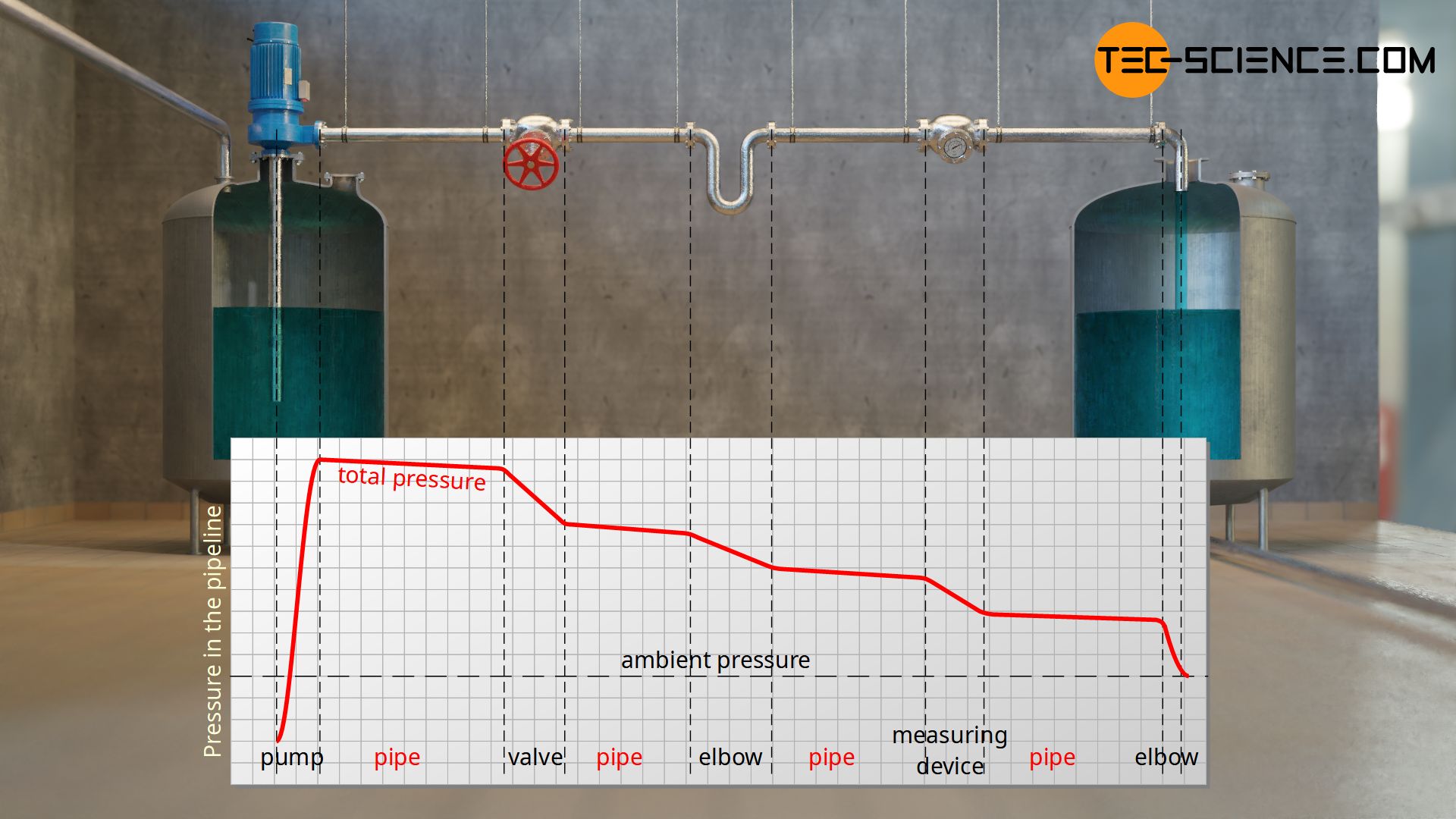
The pressure loss basically refers to the loss of static pressure (or loss of total pressure). The dynamic and hydrostatic pressure are not affected by the energy losses, as these are only the effect of the flow but not the cause. The hydrostatic pressures and dynamic pressures are predetermined by the geometry of the pipeline. Further pressure losses occur in individual components, e.g. valves, elbows or measuring equipment.
The (static) pressure loss in pipelines is associated with the loss of mechanical energy that inevitably occurs when a fluid flows through a pipe system.
In the following, we only consider incompressible flows such as liquids or slow flowing gases.
Pressure loss in pipes (Darcy friction factor)
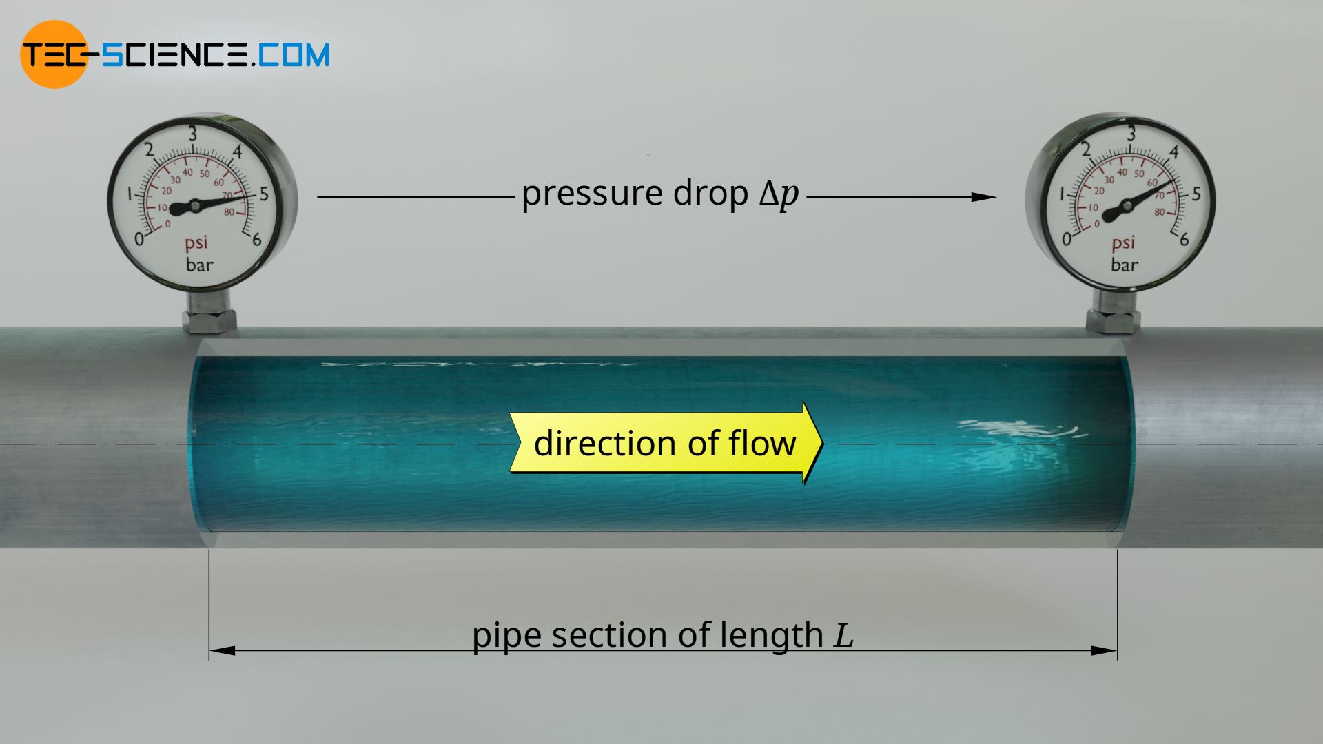
Regardless of whether the flow is laminar or turbulent, the pressure loss or pressure drop through a pipeline is described by a dimensionless similarity parameter. This so-called Darcy friction factor f basically describes the relationship between pressure loss Δpl (energy loss) and the kinetic energy contained in the flow in the form of the dynamic pressure Δpdyn. In addition, the ratio of inner pipe diameter d and pipe length L must be taken into account.
\begin{align}
& f:= \frac{\Delta p_\text{l}}{p_\text{dyn}} \cdot \frac{d}{L}~~~\text{where}~~~ p_\text{dyn}=\tfrac{1}{2}\rho ~\bar v^2 ~~~\text{:} \\[5px]
\label{lambda}
& \boxed{f= \frac{\Delta p_\text{l}}{\tfrac{1}{2}\rho ~\bar v^2} \cdot \frac{d}{L}} ~~~\text{Darcy friction factor (resistance coefficient)} \\[5px]
\end{align}
In this equation d denotes the inside diameter of the pipe and L the length of the straight pipe section along which the pressure drop is Δpl. The Darcy friction factor is also referred to as resistance coefficient or just friction factor.
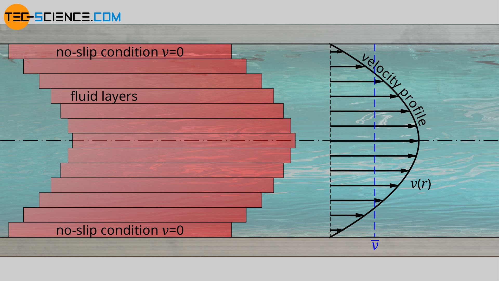
The flow velocity refers to the mean flow velocity of the fluid in the pipe. Note that in both turbulent and laminar flow there is no uniform velocity distribution across the pipe cross section, but a typical velocity profile (see Poiseuille flow).
The Darcy friction factor (resistance coefficient) is a dimensionless similarity parameter to describe the pressure loss in straight pipe sections!
By defining the friction factor as a similarity parameter, the friction factor can be determined in a reduced model scale of the later pipe system. This can then be applied to the real scale and thus the pressure loss in the actual pipeline can be determined:
\begin{align}
\label{def}
& \boxed{\Delta p_\text{l} = f \cdot \frac{1}{2}\rho ~\bar v^2 \cdot \frac{L}{ d}} ~~~\text{pressure loss in a straight pipe section} \\[5px]
\end{align}
The friction factor can also be calculated mathematically based on the geometry of the pipe, as will be shown later.
Note that this formula only applies to straight pipe sections. In pipe elbows, further losses usually occur due to the redirection of the flow, which leads to pressure losses. These component-dependent pressure losses (individual resistances) are taken into account separately by a minor loss coefficient ζ. More about this later.
In practice, often not a certain flow velocity is required, but a certain volumetric flow rate. The mean flow velocity v is linked to the volume flow rate V* by the cross-sectional area of the pipe A:
\begin{align}
&\boxed{\dot V =\bar v \cdot A} ~~~\text{where}~A=\frac{\pi}{4}d^2~~~\text{:} \\[5px]
&\dot V = \bar v \cdot \frac{\pi}{4}~d^2 \\[5px]
\label{vol}
&\underline{\bar v = \frac{4\dot V}{\pi ~d^2}} \\[5px]
\end{align}
If equation (\ref{vol}) is used in equation (\ref{def}), then the following formula for the pressure loss at a given volume flow rate is finally obtained:
\begin{align}
& \Delta p_\text{l} = f \cdot \frac{1}{2}\rho ~\left( \frac{4\dot V}{\pi ~d^2}\right)^2 \cdot \frac{L}{ d}\\[5px]
\label{volu}
& \boxed{\Delta p_\text{l} = f \cdot \frac{8\rho~L}{\pi^2} \cdot \frac{\dot{V}^2}{d^5}} ~~~\text{pressure loss in a straight pipe section} \\[5px]
\end{align}
The diameter obviously influences the pressure loss to the fifth power and thus has a decisive influence. In general, the larger the diameter, the lower the pressure loss! Note that the friction factor f is, however, dependent on the flow velocity. The flow velocity in turn depends on the volumetric flow rate and thus on the pipe diameter! So, these variables generally influence each other.
Pressure loss for laminar flow
The pressure loss resulting from the viscosity due to the internal friction of the fluid (“toughness”) has already been derived in detail for a laminar flow in the article on the Hagen-Poiseuille equation:
\begin{align}
\label{lam}
& \boxed{\Delta p_\text{l,lam} = \frac{32~\eta ~ L}{d^2} \cdot \bar v} ~~~\text{pressure loss due to viscosity} \\[5px]
\label{lam2}
& \boxed{\Delta p_\text{l,lam} = \frac{128~\eta ~ L}{\pi d^4} \cdot \dot V} \\[5px]
\end{align}
In this equation Δpl,lam denotes the pressure drop along a pipe section with the inside diameter d and the length L when a fluid with the dynamic viscosity η flows laminar through the pipe with the mean velocity v or the volume flow rate V*.
The pressure loss that inevitably occurs due to the ever-present viscosity of fluids must be compensated in any case if a fluid is to be pumped through a pipe. The pressure loss therefore corresponds to the pressure that a pump must generate in any case to keep the fluid flowing.
The Darcy friction factor flam for a laminar pipe flow can be determined by using formula (\ref{lam}) in equation (\ref{lambda}):
\begin{align}
\require{cancel}
f_\text{lam} &= \frac{\Delta p_\text{l,lam}}{\tfrac{1}{2}\rho ~\bar v^2} \cdot \frac{d}{L}\\[5px]
&= \frac{\frac{32~\eta ~ L}{d^2} \cdot \bar v}{\tfrac{1}{2}\rho ~\bar v^2} \cdot \frac{d}{L}\\[5px]
&= \frac{2 \cdot 32~\eta ~ \cancel{L}~\cancel{\bar v}}{d^{\cancel{2}}~\rho ~\bar v^{\cancel{2}}} \cdot \frac{\cancel{d}}{\cancel{L}}\\[5px]
&= \frac{64~\eta}{d~\rho ~\bar v}\\[5px]
&= \dfrac{64}{\color{red}{\dfrac{d \rho ~\bar v}{\eta}}}~~~\text{mit}~~~\color{red}{Re=\frac{d~\rho~\bar v}{\eta}}\\[5px]
\end{align}
\begin{align}
\label{a}
&\boxed{f_\text{lam}= \dfrac{64}{Re}} ~~~\text{Darcy friction factor for laminar flow}\\[5px]
\end{align}
With laminar flow, the friction factor depends only on the Reynolds number. The higher the Reynolds number, the lower the friction factor!
Note that although the friction factor decreases with increasing flow velocity (increasing Reynolds number), this does not mean that the pressure loss is reduced. According to equation (\ref{def}), the pressure loss increases with the second power of the flow velocity. The pressure loss thus increases proportionally with the flow velocity – see equation (\ref{lam})!
It has already been said that friction is not only present within the fluid itself, but that friction effects also occur in general between the fluid and the pipe wall. However, since the fluid adheres to the wall anyway (no-slip condition) and the laminar layers cover the roughness of the wall, this has no additional influence on the pressure loss. The total pressure loss is therefore given only by equation (\ref{a}) for a laminar flow. The situation is different for turbulent flows, which will be discussed in more detail in the next section.
Pressure loss for turbulent flow
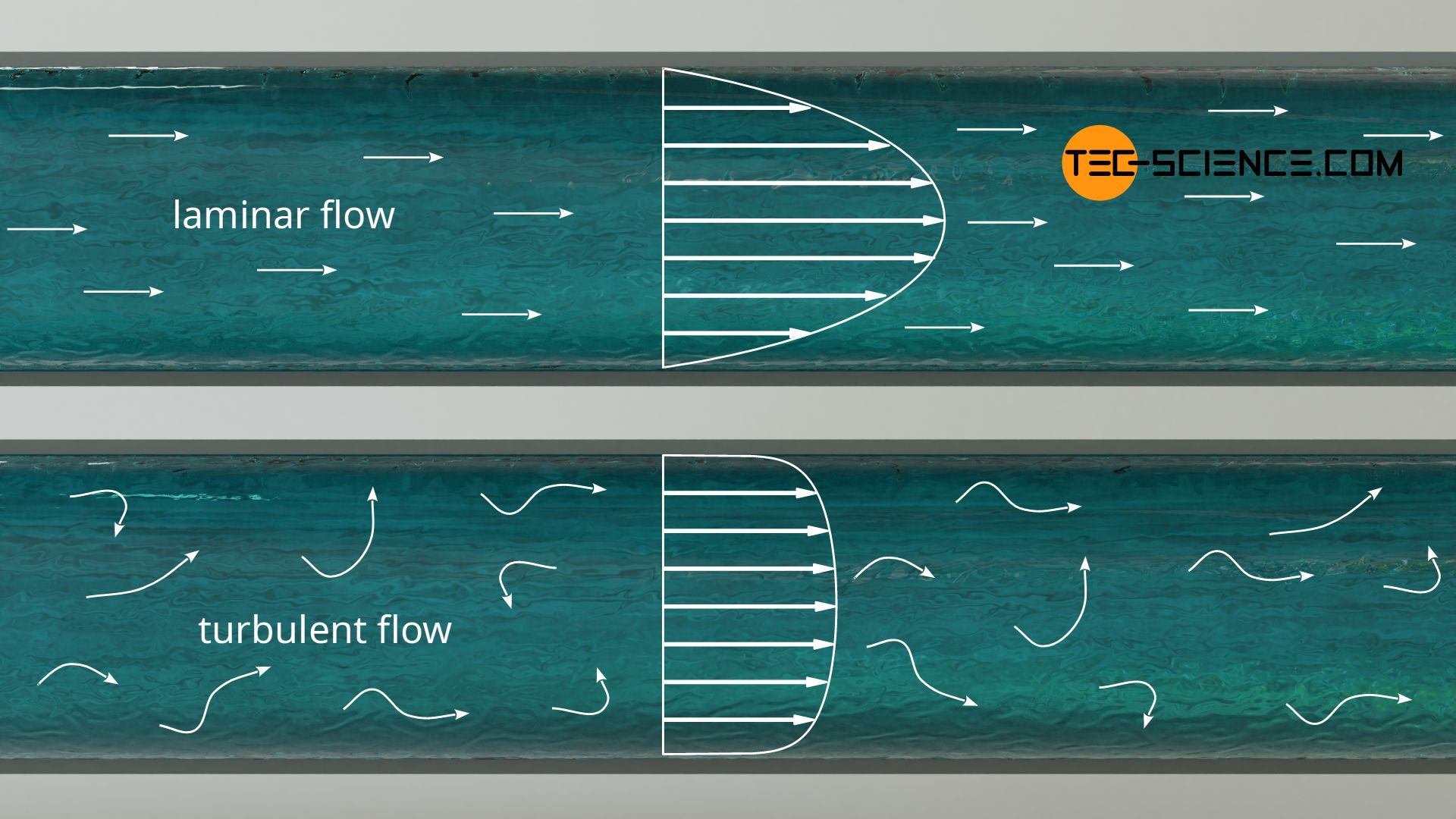
Turbulence in a flow means a lot of vortices. These contain kinetic energy, but this energy is not really transported. Downstream, this energy does not find its way, so to speak, and is therefore lost in a technically sense. In addition to the pressure loss due to internal friction caused by the viscosity of the fluid, there is therefore an additional pressure loss due to the turbulence. The pressure loss is therefore greater in turbulent flow than in laminar flow.
Viscous sublayer
In turbulent flows, the roughness of the pipe wall has a great influence on the friction factor. For this purpose we take a closer look at the situation of the fluid on the rough pipe wall. First of all, even in turbulent flows, the fluid particles located directly on the wall adhere to it due to the no-slip condition. However, no turbulence can form in the immediate vicinity of the wall, as cross-flows are prevented by the wall (the fluid cannot flow through the wall). For this reason, a so-called laminar sublayer, also referred to as viscous sublayer, forms directly at the wall.
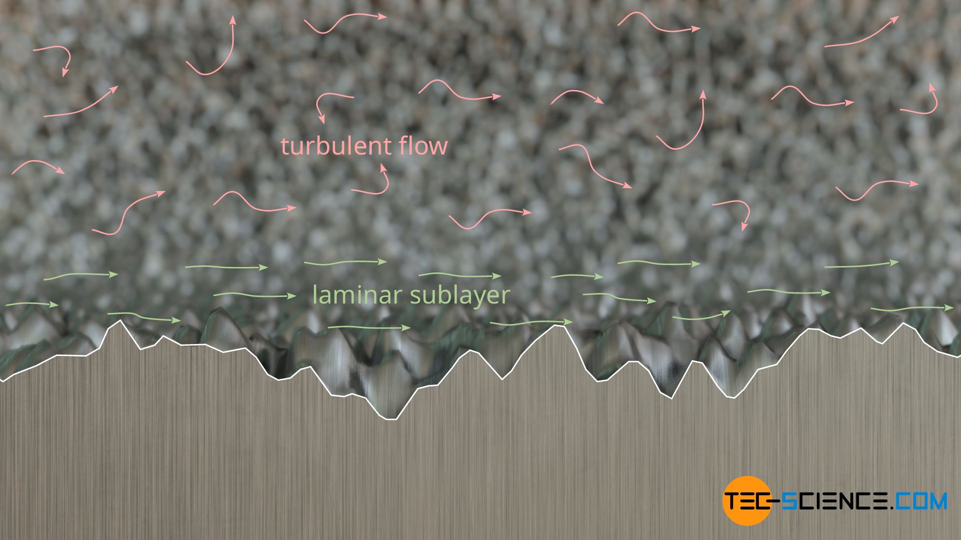
Depending on how thick this viscous sublayer is and how large the roughness is, the sublayer covers the roughness of the wall more or less. If the roughnesses are too large, then they influence the flow very strongly and lead to increased turbulence. These in turn cause a relatively large pressure loss. If, on the other hand, the surface roughness protruding from the viscous sublayer is relatively small, then the turbulence and thus the pressure loss is lower. If, on the other hand, the surface roughnesses are completely covered by the viscous sublayer, then the pressure loss due to the turbulence in the flow is lowest. In this case one also speaks of a hydraulically smooth pipe.
A pipe is considered hydraulically smooth when the viscous sublayer completely covers the surface roughness. The pressure loss is lowest in this case!
Relative roughness
The roughness of a surface is indicated by a roughness parameter k (also denoted by Rz). This roughness parameter describes the height between the lowest and highest points of a rough surface, averaged over several sections.
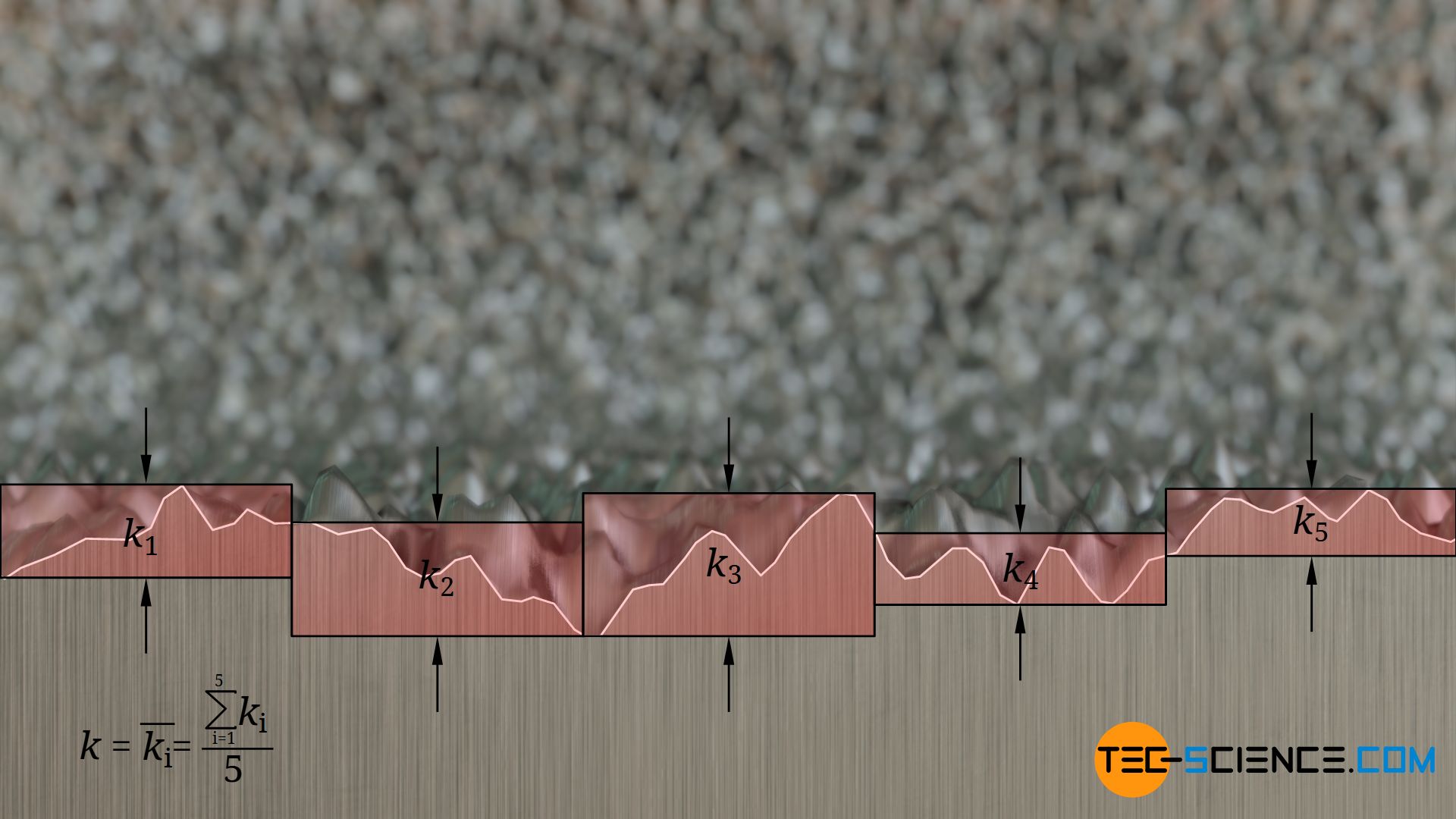
However, this roughness parameter as an absolute measure of the roughness of the pipe wall is not suitable for characterizing the influence on the turbulent flow. The roughness must always be considered in relation to the entire flow cross-section, i.e. the inner diameter of the pipe. The ratio of absolute roughness k and pipe diameter d is also called relative roughness ε:
\begin{align}
\label{e}
&\boxed{\varepsilon= \frac{k}{d}} ~~~\text{relative roughness}\\[5px]
\end{align}
The relative roughness indicates the percentage of the total pipe diameter taken up by the roughness.
Implicit Colebrook-White equation
The scientists Colebrook and White derived the following implicit function for determining the Darcy friction factor ftur for turbulent pipe flows using empirical results:
\begin{align}
\label{cw}
&\boxed{\color{red}{\frac{1}{\sqrt{f_\text{tur}}}}=-2\cdot \log_\text{10}\left(\frac{2.51}{Re} \cdot \color{red}{\frac{1}{\sqrt{f_\text{tur}}}} +\frac{\varepsilon}{3.71}\right)} ~~~\text{Colebrook-White equation} \\[5px]
\end{align}
The term “implicit” means that this equation cannot be solved directly for the friction factor. Rather, with a given Reynolds number Re of the flow and a given relative roughness ε of the pipe wall, it is necessary to find a friction factor which then satisfies this equation. If this is the case, the friction factor found corresponds to the value searched for. In the next section Explicit Haaland equation, an iterative solution of this equation is described in more detail. With a so-called Moody chart, the friction factors can also be determined graphically.
For hydraulically smooth pipes, the viscous sublayer covers the roughness of the wall. In this case, the relative roughness ε in the Colebrook-White equation must be set to zero, regardless of the value actually obtained:
\begin{align}
&\boxed{\color{red}{\frac{1}{\sqrt{f_\text{tur}}}}=-2\cdot \log_\text{10}\left(\frac{2.51}{Re} \cdot \color{red}{\frac{1}{\sqrt{f_\text{tur}}}} \right)} ~~~\text{for hydraulically smooth pipes} \\[5px]
\end{align}
If the surface roughness of the pipe wall protrude completely from the viscous sublayer, the friction factor is determined almost exclusively by the wall roughness and is independent of the Reynolds number. The scientist Nikuradze derived the following explicit equation for such hydraulically rough pipes to determine the pipe friction coefficient:
\begin{align}
&\boxed{\color{red}{\frac{1}{\sqrt{f_\text{tur}}}}=-2\cdot \log_\text{10}\left(\frac{\varepsilon}{3.71} \right)} ~~~\text{for hydraulically rough pipes} \\[5px]
&f_\text{tur}=\frac{1}{\left[2\cdot \log_\text{10}\left(\frac{3.71}{\varepsilon} \right)\right]^2} \\[5px]
\end{align}
Explicit Haaland equation
There is a reason why the Colebrook-White equation (\ref{cw}) is given in this somewhat strange form. This allows an iterative procedure, so that the friction factor can be determined starting from a starting value 1/√ftur,0. The starting value can be determined by the explicit equation proposed by Haaland:
\begin{align}
&\boxed{\color{red}{\frac{1}{\sqrt{f_\text{tur,0}}}}=-1.8\cdot \log_\text{10}\left(\frac{6.9}{Re} +\left(\frac{\varepsilon}{3,7}\right)^{1.11}\right)} ~~~\text{Haaland equation} \\[5px]
\end{align}
The value 1/√ftur,0 explicitly determined with the Haaland equation can now be used in the right side of the Colebrook-White equation. This results in a new value 1/√ftur,1 according to the left side of the equation. This value can then again be used in the right side of the equation. The value 1/√ftur,2 obtained after two passes usually corresponds with sufficient accuracy to the value 1/√ftur searched for. Finally, the pipe friction coefficient ftur can be determined.
Alternatively to the Haaland equation, a value of 1/√ftur,0=7.5} can be used as a starting value. This corresponds to the result of the Haaland equation for a hydraulically smooth pipe (ε=0) and a Reynolds number of 105.
Power loss
Any pressure loss in a pipeline must be compensated by the power of an appropriate pump. The power loss Pl due to the pressure loss Δpl depends on the volume flow rate V*:
\begin{align}
\label{v}
&P_\text{l} = \Delta p_\text{l} \cdot \dot V \\[5px]
\end{align}
If the pressure drop Δpl according to equation (\ref{volu}) is put in equation (\ref{v}), then the following formula results:
\begin{align}
\label{dr}
&\boxed{P_\text{l} = f \cdot \frac{8\rho~L}{\pi^2} \cdot \frac{\dot{V}^3}{d^5}} ~~~\text{applies in general}\\[5px]
\end{align}
At this point it must again be noted that the friction factor f is dependent on the Reynolds number and thus on the flow velocity. The flow velocity, in turn, depends on the volume flow rate and the pipe diameter!
Only for laminar flows, there is an explicit relationship between the Reynolds number and the friction factor according to equation (\ref{a}). In this case, the pressure loss for laminar flows can be directly put into the formula for the power loss (\ref{v}) according to equation (\ref{lam2}). In the case of laminar pipe flows, the following relationship then applies:
\begin{align}
&P_\text{l,lam} = \Delta p_\text{l,lam} \cdot \dot V \\[5px]
&\boxed{P_\text{l,lam} = \frac{128~\eta ~ L}{\pi} \cdot \frac{\dot{V}^2}{d^4}} ~~~\text{only applies to laminar flows}\\[5px]
\end{align}
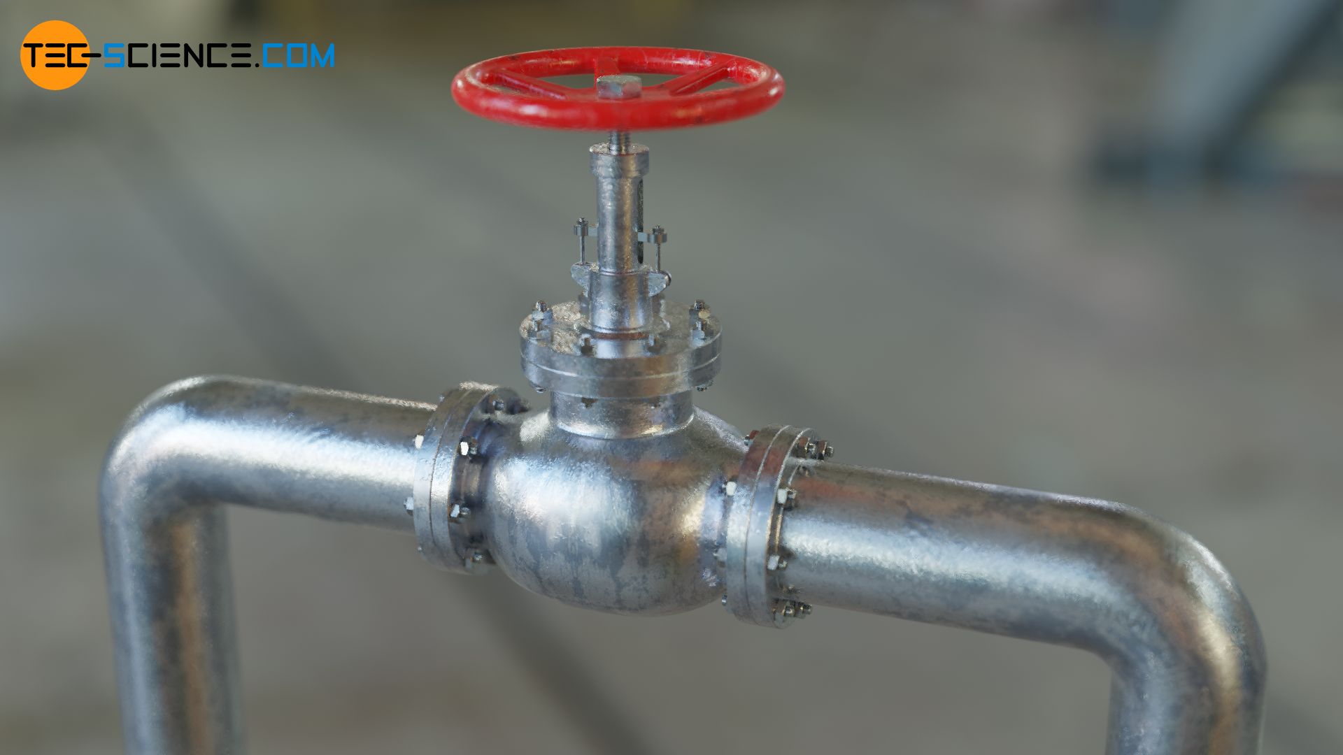
Pressure loss through individual components (minor loss coefficient)
A pipe system usually does not consist of a single straight pipe. A pipe system usually consists of several elbows, branches, reducers, valves, etc. These individual components also cause energy losses and thus pressure losses.
These pressure losses are each described by a minor loss coefficient ζ. The minor loss coefficient is defined analogously to the Darcy friction factor, i.e. as the ratio between pressure loss Δpl in the component and the dynamic pressure of the flow pdyn:
\begin{align}
& \zeta:= \frac{\Delta p_\text{l}}{p_\text{dyn}} ~~~\text{where}~~~ p_\text{dyn}=\tfrac{1}{2}\rho ~\bar v^2 ~~~\text{:} \\[5px]
\label{zeta}
& \boxed{\zeta= \frac{\Delta p_\text{l}}{\tfrac{1}{2}\rho ~\bar v^2} } ~~~\text{minor loss coefficient} \\[5px]
\end{align}
The meaning of the minor loss coefficient for objects through which a fluid flows is ultimately identical to the drag coefficient for bodies around which flow passes.
The minor loss coefficient is a dimensionless similarity parameter to describe the pressure loss in individual components (elbows, valves, reducers, etc.)!
The minor loss coefficients for the various components are usually determined experimentally and are given in table books. If the minor loss coefficient is known, the pressure loss through the component can then be determined as follows:
\begin{align}
\label{dez}
& \boxed{\Delta p_\text{l} = \zeta \cdot \frac{1}{2}\rho ~\bar v^2 } ~~~\text{pressure loss in individual components} \\[5px]
\end{align}
The flow velocity basically refers to the velocity of the fluid prior to the actual component and not to the flow velocity inside the component! A valve, for example, reduces the flow cross-section and thus increases the flow speed in the component. However, the flow velocity to be taken as a basis for the pressure loss refers to the flow velocity in the pipeline!
Eventually a minor loss coefficient can even be defined for a straight pipe section. In this way the straight pipe sections can also be considered as single component. In this case the minor loss coefficient is related to the Darcy friction factor f and the length of the pipe section L and the internal pipe diameter d as follows:
\begin{align}
&\boxed{\zeta_\text{p} = \frac{L}{d} f}~~~\text{minor loss coefficient of a straight pipe section} \\[5px]
\end{align}
Conversely, a so-called equivalent pipe length Le can be given for individual components. These components can then be imagined as additional pipe sections. In the equation given below, the Darcy friction factor f corresponds to the friction factor of the actual pipes.
\begin{align}
&\boxed{L_\text{e}= \frac{d \cdot \zeta}{f}}~~~\text{equivalent pipe length of components} \\[5px]
\end{align}
With a pipe diameter of d = 1 cm, a minor loss coefficient of ζ=1 and a friction factor of f = 0.02, an equivalent pipe length of only 0.5 m is obtained. With very long piping systems and only few individual components (which is often the case), the pressure loss due to the installed components can therefore usually be neglected. For this reason, the resistance coefficient for individual components is called the minor loss coefficient. But note: In some cases the minor loss coefficient can have an enormous effect, especially for short piping systems!
In general, the following therefore applies: The sum of the pressure losses Δpl.p through the individual straight pipe sections, plus the sum of the pressure losses Δpl,c through the individual components, gives the total pressure loss Δpl,total of the entire pipe system:
\begin{align}
&\boxed{\Delta p_\text{l,total} = \sum \Delta p_\text{l,p} +\sum \Delta p_\text{l,c} } \\[5px]
\end{align}
For only one pipeline of total length L with constant inside diameter d and thus constant mean flow velocity v the following formula applies:
\begin{align}
&\boxed{\Delta p_\text{l,total} = \left(f \frac{L}{d} + \sum \zeta \right) \frac{1}{2}\rho~\bar{v}^2} \\[5px]
\end{align}
")


")
")
