Equation of motion of a fluid on a streamline

In this article we derive the equation of motion of a fluid element on a streamline and one perpendicular to it.

Introduction

In the following we want to derive the equation of motion of a fluid element on a streamline for a plane, laminar flow (two-dimensional flow). For example, one can imagine a flow in a curved, deep channel, which is viewed from above. We define a fixed coordinate system s in a horizontal plane parallel to the earth’s surface, which runs in the direction of the streamline. The radius of curvature of the streamline is denoted by r_c.

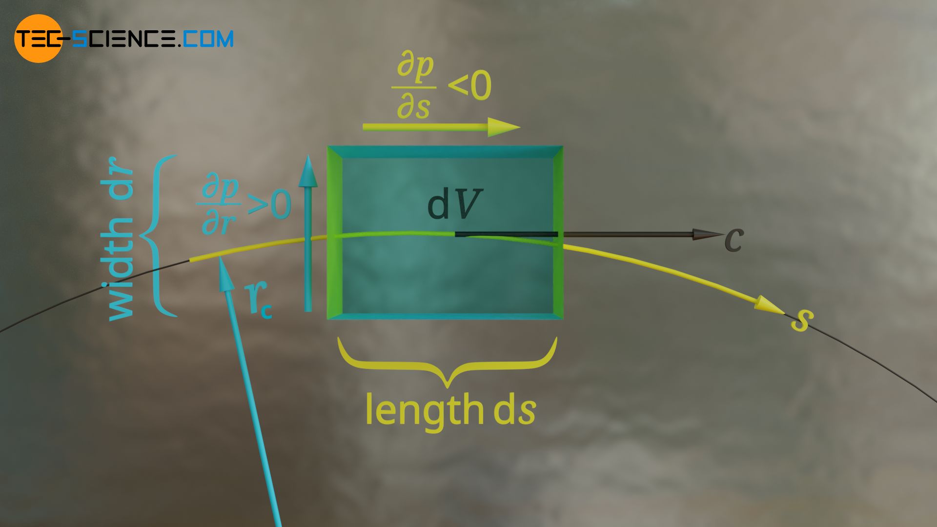
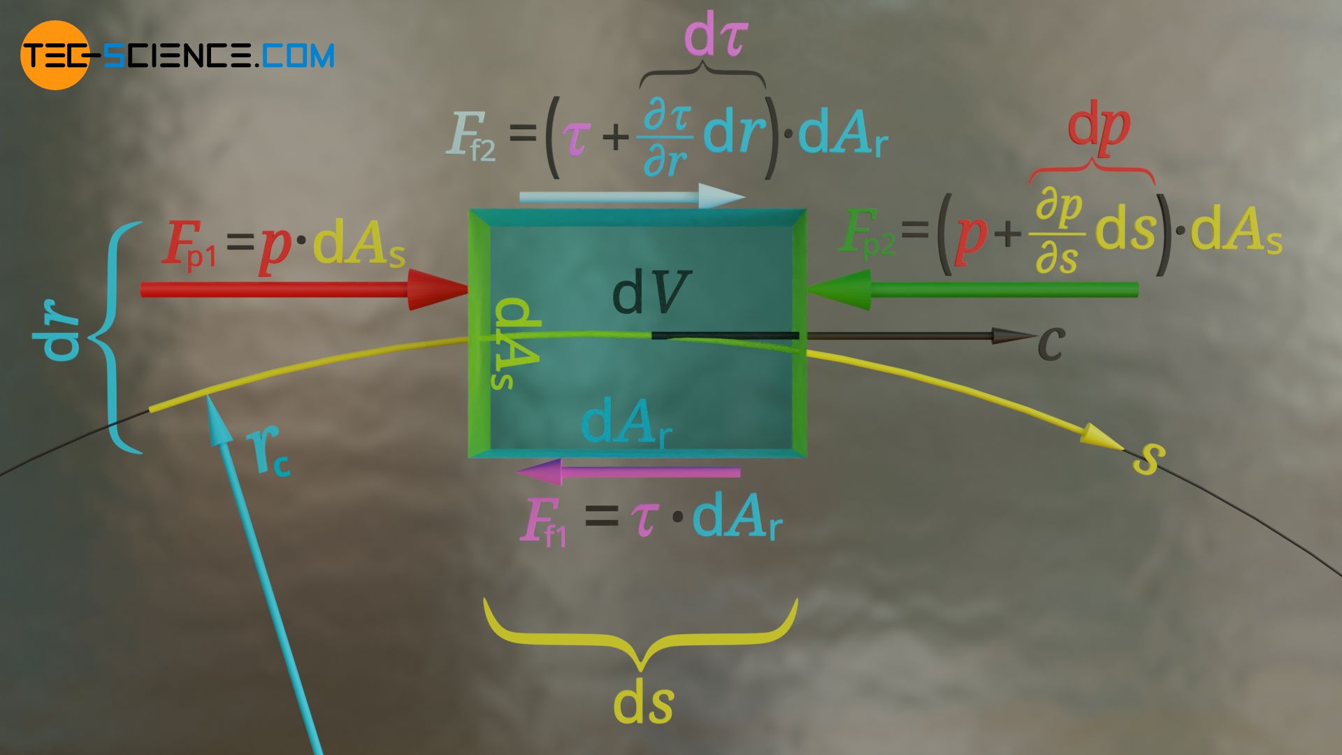
The fluid element has the width dr in radial direction and the length ds in direction of the streamline. The pressure gradient in the direction of the streamline is ∂p/∂s<0 and in radial direction ∂p/∂r>0. The fluid element with the volume dV moves with the velocity c on the streamline.

Equation of motion of a fluid element in the direction of the streamline

Substantial acceleration

First, we consider the kinetics of a fluid element only in the direction of the streamline. By definition, the fluid element moves at the velocity c tangential to the streamline. Since, however, in the case of a unsteady flow, the flow velocity c not only varies from place to place, but also changes over time at a fixed location (e.g. when the flow “starts”), the acceleration of a fluid element is basically made up of two parts:

1. the temporal change of velocity at a fixed location (local acceleration) and
2. the spatial change of velocity from place to place (convective acceleration).

The first part results from the fact, that every temporal change of speed at a fixed location represents an acceleration. This means: If the speed of the fluid element changes at a fixed location, this can only be a consequence of a respective acceleration. The second part is due to the fact that the speed not only changes in time at a fixed location, but also differs from place to place at a certain point in time. This means that a fluid element must be accelerated to the new flow velocity, so to speak, when its location changes. Both parts together represent the so-called substantial acceleration, i.e. the acceleration which actually acts on the fluid element as a whole (also called material acceleration).

The substantial change of the velocity dc is thus obtained by a temporal change of the velocity ∂c/∂t within the time dt and by a spatial change of the velocity ∂c/∂s (gradient) within a distance ds:

\begin{align}
&\underbrace{\text{d}c}_{\text{substantial change}} = \underbrace{\frac{\partial c}{\partial t} \text{d}t}_{\text{local change}} + \underbrace{\frac{\partial c}{\partial s} \text{d}s}_{\text{convective change}}\\[5px]
\end{align}

If this equation is divided by the time dt, the following formula for the substantial acceleration a_t in tangential direction of the streamline is obtained:

\begin{align}
&a_t = \frac{\text{d}c}{\text{d}t} = \frac{\partial c}{\partial t} + \frac{\partial c}{\partial s} \underbrace{\frac{\text{d}s}{\text{d}t}}_{c}\\[5px]
& \underline{a_t = \frac{\partial c}{\partial t} + c\frac{\partial c}{\partial s}} \\[5px]
\end{align}

Note, that the term of convective acceleration depends on the flow velocity. This is also clear, because if the fluid element flows very fast, it covers a relatively long distance within a certain time. For a given velocity gradient ∂c/∂s this means a correspondingly large change in velocity and thus a large acceleration.

Thus the following accelerating tangential force F_t acts on a considered fluid element of mass dm in streamline direction, whereby the mass can be expressed by the volume of the fluid element dV and the density ϱ:

\begin{align}
\label{t}
& \boxed{F_t = \text{d}m \cdot a_t = \text{d}V \cdot \rho \cdot \left( \frac{\partial c}{\partial t} + c\frac{\partial c}{\partial s}\right)} ~~~~~\text{accelerating tangential force} \\[5px]
\end{align}

Pressure forces

The upper equation only describes the effect of a local and temporal change in velocity on acceleration (kinematics), but not the cause of this acceleration (kinetics). The cause of the accelerating force are the forces acting on the fluid element. We would therefore have to take a closer look at and balance the forces acting on the fluid element. Here, too, we will only consider the motion or forces in the direction of the streamline.

Forces act on the end faces of the fluid element due to the pressure acting there, which decreases along the streamline. Note that a fluid particle can only move in the direction of decreasing pressure, because a decreasing pressure gradient ∂p/∂s<0 is what drives a flow in the first place. So if a pressure p acts on the left end side dA_s, then at the right end side (over the distance ds), there ist a pressure lower by p+∂p/∂s⋅ds:

\begin{align}
& \underline{F_{p1} = p \cdot \text{d}A_s} \\[5px]
& \underline{F_{p2} = \left(p+\frac{\partial p}{\partial s}\cdot \text{d}s \right) \cdot \text{d}A_s} \\[5px]
\end{align}

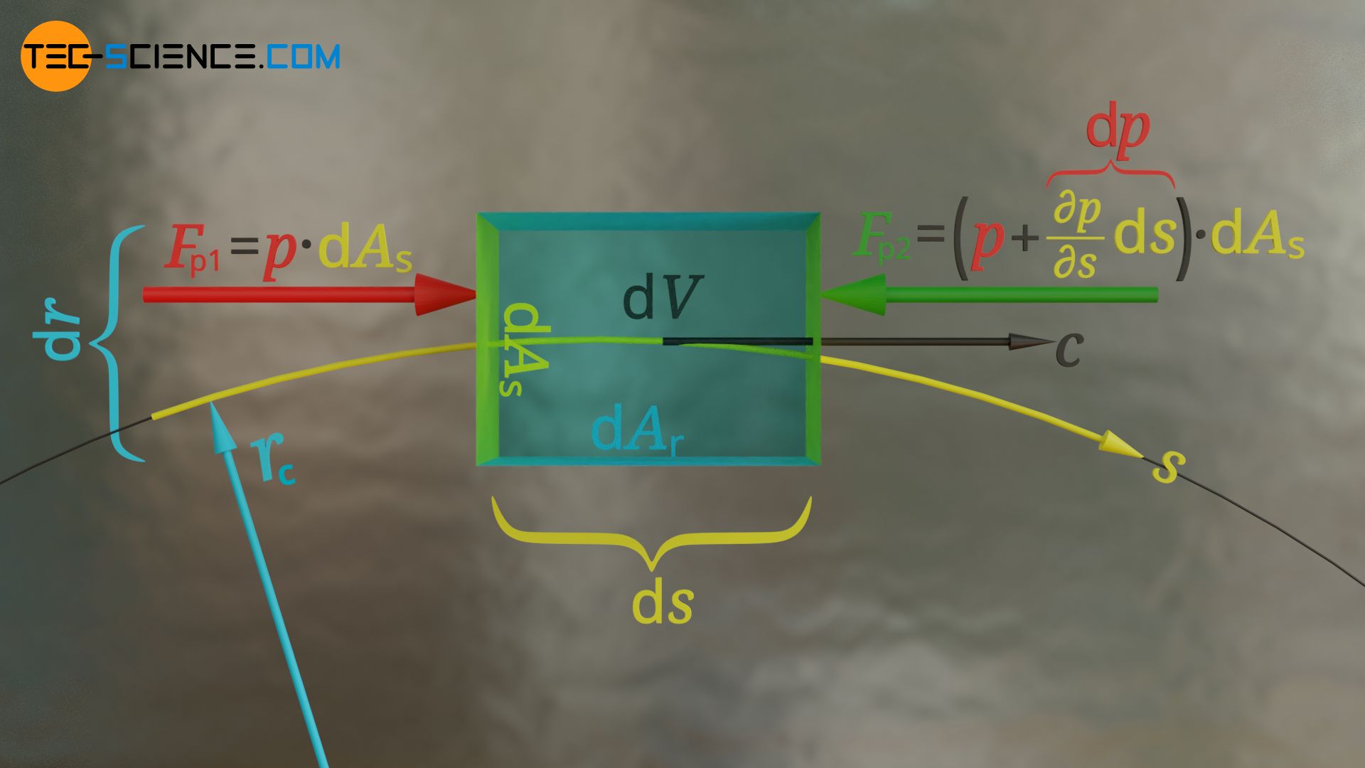
The resultant pressure force acting on the fluid element F_p finally results from the difference between the two forces:

\begin{align}
\require{cancel}
F_p &= F_{p1} – F_{p2} \\[5px]
&=p \cdot \text{d}A_s – \left(p+\frac{\partial p}{\partial s}\cdot \text{d}s \right) \cdot \text{d}A_s \\[5px]
&=\cancel{p \cdot \text{d}A_s} – \cancel{p \cdot \text{d}A_s} – \frac{\partial p}{\partial s}\cdot \underbrace{\text{d}s \cdot \text{d}A_s}_{\text{d}V} \\[5px]
\end{align}

\begin{align}
\boxed{F_p = – \frac{\partial p}{\partial s}\cdot \text{d}V}~~~~~\text{resultant pressure force} \\[5px]
\end{align}

Frictional forces

Furthermore, frictional forces act on the lateral faces due to the dynamic viscosity η of the fluid. These can be determined using Newton’s law of friction for fluids:

\begin{align}
\label{n}
& \tau= \eta \cdot \frac{\partial c}{\partial r} \\[5px]
\end{align}

In this equation τ denotes the shear stress acting in the surface, which is proportional to the radial velocity gradient ∂c/∂r. This velocity gradient describes the spatial change in velocity perpendicular to the streamline. However, across the width dr of the fluid element, this velocity gradient changes in general. Thus, different shear stresses act on both sides.

If ∂τ/∂r denotes the change of the shear stress in radial direction (shear stress gradient), then for a given width of the fluid element of dr the shear stress changes by the amount ∂τ/∂r⋅dr. For the laterally acting shear forces the following formulas therefore apply:

\begin{align}
& F_{f1} = \tau \cdot \text{d}A_r \\[5px]
& F_{f2} = \left(\tau+ \frac{\partial \tau}{\partial r}\text{d}r\right) \cdot \text{d}A_r \\[5px]
\end{align}

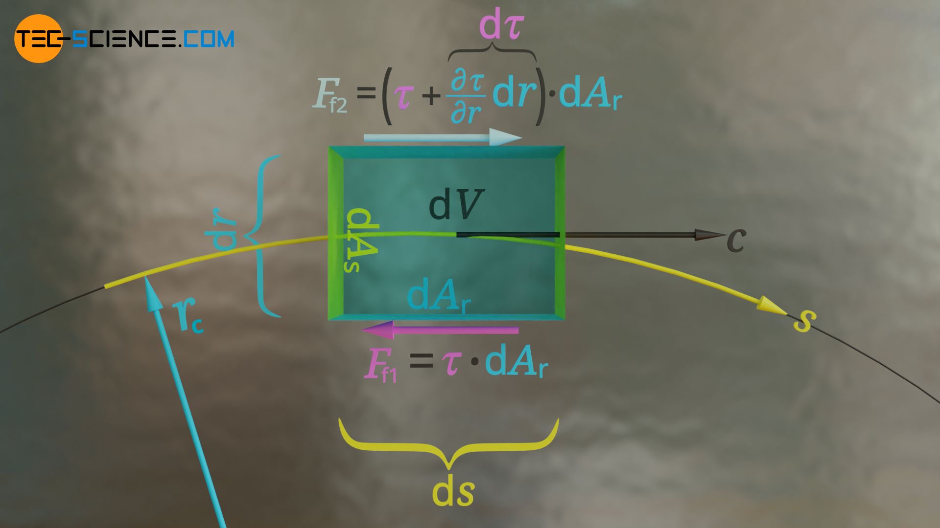
Note that the forces acting laterally are pointing in different directions. If we assume that the flow velocity increases in the radial direction, the surrounding fluid on the right side (viewed in the direction of flow) flows at a lower velocity than the fluid element. The fluid element is slowed down, so to speak, and the force is accordingly directed against the flow direction. On the opposite left side, the surrounding fluid flows faster than the fluid element. The surrounding fluid tries to “drag” the fluid element along, so to speak, and the force therefore acts in the direction of flow.

If at this point the shear stresses occurring in the upper equations are expressed by Newton’s law of friction according to equation (\ref{n}), then the following relationship is obtained for the laterally acting shear forces (friction forces):

\begin{align}
&\underline{F_{f1} = \eta \cdot \frac{\partial c}{\partial r} \cdot \text{d}A_r} \\[5px]
\end{align}

\begin{align}
F_{f2} &= \left(\eta \cdot \frac{\partial c}{\partial r}+ \frac{\partial}{\partial r}\left(\eta \cdot \frac{\partial c}{\partial r}\right) \text{d}r\right)\cdot \text{d}A_r \\[5px]
&= \left(\eta \cdot \frac{\partial c}{\partial r}+ \eta \cdot \frac{\partial}{\partial r}\left(\frac{\partial c}{\partial r}\right) \text{d}r\right)\cdot \text{d}A_r \\[5px]
\end{align}

\begin{align}
&\underline{F_{f2}= \eta \left(\frac{\partial c}{\partial r}+ \frac{\partial^2 c}{\partial r^2}~\text{d}r\right) \cdot \text{d}A_r} \\[5px]
\end{align}

All frictional forces on the fluid element are now mathematically described. Note that there are no frictional forces acting perpendicular to the considered horizontal plane (i.e. on the top and bottom side of the fluid element), since there is no velocity gradient in the vertical direction in a plane flow (spatially constant velocity). And if there is no velocity gradient, then according to Newton’s law of friction there is no friction. This is also clear, because if the velocity of the fluid layers is identical in the vertical direction, then these do not move relative to each other and thus do not generate friction forces or cause any transfer of momentum.

The resultant frictional force F_f acting on the fluid element ultimately results from the difference between the two opposing forces:

\begin{align}
\require{cancel}
F_{f} &= F_{f2} – F_{f1} \\[5px]
&= \eta \left(\frac{\partial c}{\partial r}+ \frac{\partial^2 c}{\partial r^2}~\text{d}r\right) \cdot \text{d}A_r – \eta \cdot \frac{\partial c}{\partial r} \cdot \text{d}A_r\\[5px]
&= \cancel{\eta \cdot \frac{\partial c}{\partial r}\cdot \text{d}A_r}+\eta \frac{\partial^2 c}{\partial r^2}~\underbrace{\text{d}r \cdot \text{d}A_r}_{\text{d}V}-\cancel{ \eta \cdot \frac{\partial c}{\partial r} \cdot \text{d}A_r}\\[5px]
\end{align}

\begin{align}
&\boxed{F_f= \eta \frac{\partial^2 c}{\partial r^2}~\text{d}V} ~~~~~\text{resultant frictional force}\\[5px]
\end{align}

Balance of forces

The sum of the forces acting on the fluid element, consisting of the pressure force F_p acting on the face side and the frictional force F_f acting on the lateral side, finally corresponds to the accelerating tangential force according to equation (\ref{t}):

\begin{align}
\require{cancel}
&F_{t} = F_{f} + F_{p} \\[5px]
&\cancel{\text{d}V} \cdot \rho \cdot \left( \frac{\partial c}{\partial t} + c\frac{\partial c}{\partial s}\right) = \eta \frac{\partial^2 c}{\partial r^2}~\cancel{\text{d}V} – \frac{\partial p}{\partial s}\cdot \cancel{\text{d}V} \\[5px]
&\frac{\partial c}{\partial t} + c\frac{\partial c}{\partial s}= \underbrace{\frac{\eta}{\rho}}_{\nu} \frac{\partial^2 c}{\partial r^2} – \frac{1}{\rho}\frac{\partial p}{\partial s} \\[5px]
&\boxed{\frac{\partial c}{\partial t} + c\frac{\partial c}{\partial s}=\nu \frac{\partial^2 c}{\partial r^2} – \frac{1}{\rho}\frac{\partial p}{\partial s}} ~~~~~\text{streamline equation in a horizontal plane}\\[5px]
\end{align}

When deriving the streamline equation it was used that the quotient of dynamic viscosity and density corresponds to the kinematic viscosity ν (small Greek letter Nu). Note that this equation only applies to a plane flow where gravity acts perpendicular to the flow plane (horizontal plane).

If, however, a flow is considered in a vertical plane, then the component of the weight force that points in the direction of the streamline must also be taken into account. In the streamline equation an additional term then occurs.

\begin{align}
\label{euler}
&\boxed{\frac{\partial c}{\partial t} + c\frac{\partial c}{\partial s}=\nu \frac{\partial^2 c}{\partial r^2} – \frac{1}{\rho}\frac{\partial p}{\partial s}-g\frac{\partial z}{\partial s}} ~~~~~\text{streamline equation in a vertical plane}\\[5px]
\end{align}

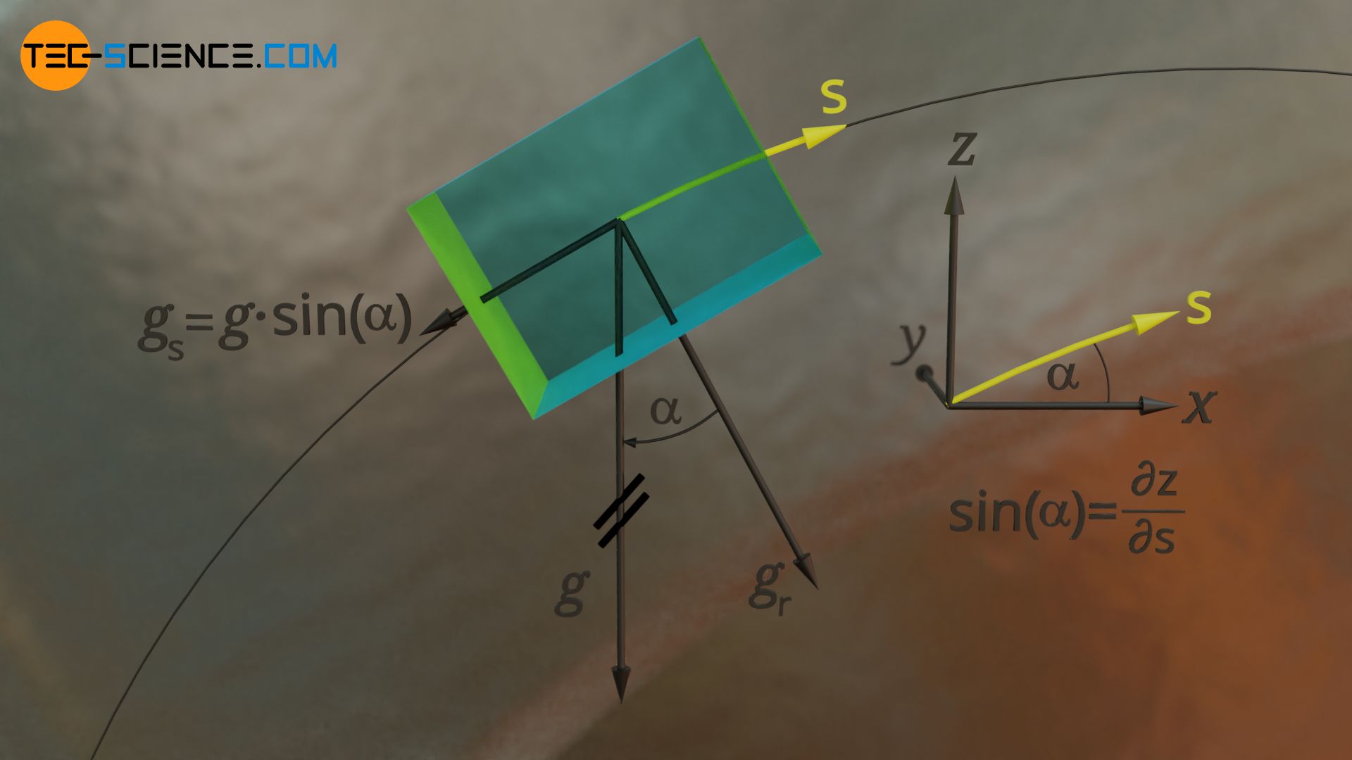
The term ∂z/∂s ultimately corresponds to the sine of the angle between the vertical axis (z-axis) and the direction of the streamline (∂z/∂s=sin(α)). The term in the equation above could therefore also be written as g⋅sin(α). Now it becomes clear that this term corresponds to the component of the weight force in the direction of the streamline.

For a horizontal flow however, obviously there is no weight component in streamline direction, so this term disappears. Both equations are further simplified if a steady flow is considered, where the flow velocities do not change in time by definition. The time derivative of the velocity is thus zero: ∂c/∂t=0 (no local acceleration, only convective acceleration)!

Equation (\ref{euler}) is actually a special case of the Euler equation, which has been extended by the term of viscosity.

Equation of motion of a fluid element perpendicular to the streamline

In this section we consider the fluid element and the forces acting perpendicular to the streamline. For the sake of simplicity, we assume a steady flow. The curved streamline can be seen as a arc section with a radius of curvature r_c. To cause such a circular path, the forces acting in the radial direction must generate a centripetal force F_c. The magnitude of this centripetal force to be applied depends on the flow velocity c, the radius of curvature r_c and the mass of the fluid element dm:

\begin{align}
&\boxed{F_c = \frac{\text{d}m \cdot c^2}{r_c}} ~~~~\text{centripetal force to be applied} \\[5px]
\end{align}

If we neglect frictional forces on the faces of the fluid element at this point, the centripetal force can only have one cause: The pressure forces on the lateral surfaces of the fluid element must be different, so that a centripetal force is generated against the radial direction. The pressure in the radial direction must therefore increase across the width of the fluid element. The quantities on which this radial pressure gradient ∂p/∂r depends are shown in the following.

The pressure increases perpendicular to the streamlines in radial direction!

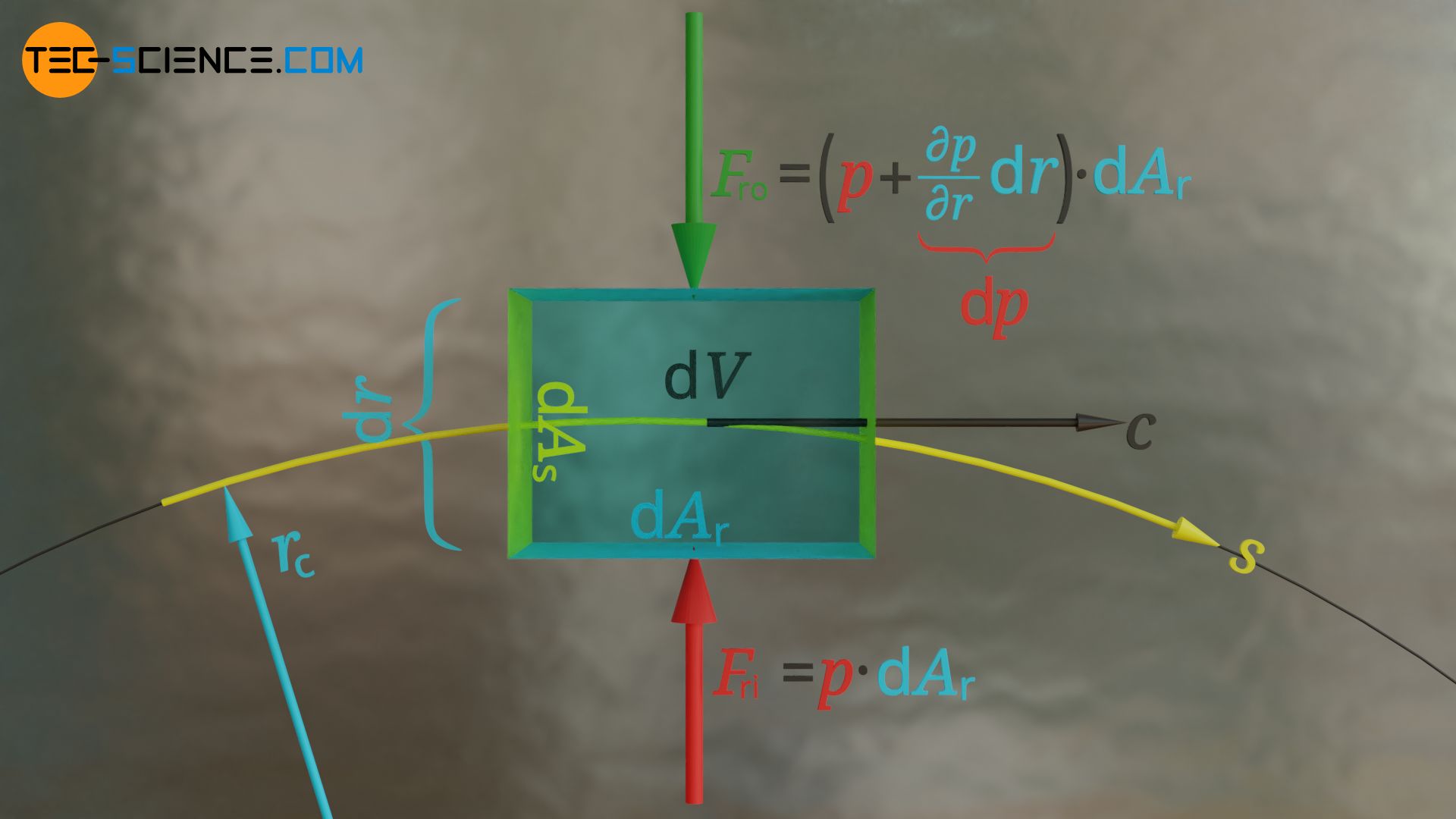
If a pressure p acts on the “inside” of the fluid element (inside regarding the curve), then for a given pressure gradient ∂p/∂r>0 a pressure lower by ∂p/∂r⋅dr results on the “outside” of the fluid element. This results in the following radial forces:

\begin{align}
& \underline{F_{ri} = p \cdot \text{d}A_r} \\[5px]
& \underline{F_{ro} = \left(p+\frac{\partial p}{\partial r}\cdot \text{d}r \right) \cdot \text{d}A_r} \\[5px]
\end{align}

The magnitude of the resultant pressure force in radial direction F_r finally results from the difference of both forces:

\begin{align}
\require{cancel}
F_r &= F_{ro} – F_{ri} \\[5px]
&= \left(p+\frac{\partial p}{\partial r}\cdot \text{d}r \right) \cdot \text{d}A_r – p \cdot \text{d}A_r \\[5px]
&= \cancel{p \cdot \text{d}A_r} + \frac{\partial p}{\partial r}\cdot \underbrace{\text{d}r \cdot \text{d}A_r}_{\text{d}V}- \cancel{p \cdot \text{d}A_r}\\[5px]
\end{align}

\begin{align}
\boxed{F_r = \frac{\partial p}{\partial r}\cdot \text{d}V}~~~~~\text{resultant radial force} \\[5px]
\end{align}

This resultant pressure force in radial direction is the cause of the centripetal force. Equating both equations finally provides the following relationship between the flow of the fluid and the resulting pressure gradient in radial direction:

\begin{align}
&F_r = F_c \\[5px]
&\frac{\partial p}{\partial r}\cdot \text{d}V = \frac{\text{d}m \cdot c^2}{r_K} \\[5px]
&\frac{\partial p}{\partial r}= \frac{\overbrace{\frac{\text{d}m}{\text{d}V}}^{\rho} \cdot c^2}{r_K} \\[5px]
&\boxed{\frac{\partial p}{\partial r}= \frac{\rho \cdot c^2}{r_K}} \\[5px]
\end{align}

The higher the flow velocity and the denser the fluid and the smaller the radius of curvature of the streamline is, the higher the pressure gradient in radial direction!

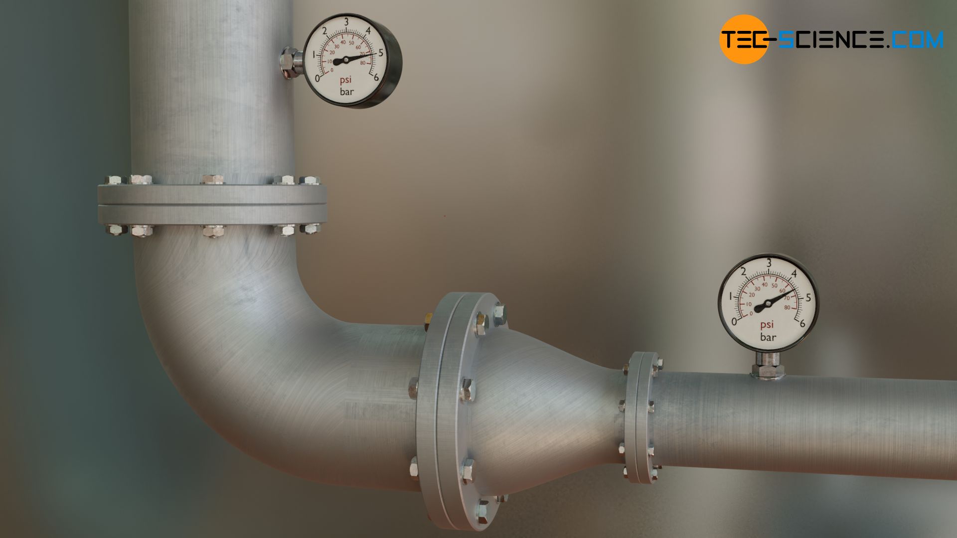
However, the above equation also shows that for large radii of curvature the radial pressure gradient becomes smaller and smaller. For straight streamlines with an infinitely large radius of curvature, the pressure gradient is infinitely small. In other words, for straight streamlines there is no pressure gradient in the radial direction.

Pressure measurements in pipes should therefore always be carried out on straight pipe sections with straight streamlines. In these cases the measured pressure is independent of the placement of the pressure gauge on the pipe circumference. When measuring pressure at pipe angles, on the other hand, the pressure varies depending on the distance from the center of curvature and thus on its placement on the circumference of the pipe.