The Maxwell-Boltzmann distribution describes the distribution of the molecular speed of the molecules in ideal gases.
Introduction
As already explained in the article Temperature and particle motion, the temperature of a gas is a measure of the kinetic energy of the particles. Even at a constant temperature, however, not all the molecules have the same speed. After all, in a gas there are permanent collisions between the particles. Some particles are slowed down by the collision and others are accelerated by it. Thus, molecules with different velocities can be found.
A gas usually contains a large number of molecules. For ideal gases, therefore, statistical predictions can be made about the frequency with which certain speeds occur. The so-called Maxwell-Boltzmann distribution describes such a speed distribution for the particles of an ideal gas.
The Maxwell-Boltzmann distribution describes the speed distribution of the particles of an ideal gas!
Such a statistical prediction about the speed distribution is only possible if a sufficient number of molecules are present. This is true in most thermodynamic cases! To get an impression of the large number of particles in an ideal gas, imagine a football filled with air. The number of gas particles in such a football would then correspond approximately to the number of 1-liter water bottles that would theoretically be necessary to completely fill the entire volume of the earth with water!

This example clearly shows that in practice a sufficiently large number of particles in a gas can usually be assumed to make reliable statistical predictions.
Maxwell-Boltzmann speed distribution
Using statistical methods, physicists James Clerk Maxwell and Ludwig Boltzmann were able to derive the following formula for the molecular speed distribution in an ideal gas. For this reason this function of the relative frequency density f(v) is also called Maxwell-Boltzmann distribution function:
\begin{align}
\label{p}
&\boxed{ f(v) = \left( \sqrt{\frac{m}{2 \pi k_B T}} \right)^{3} 4 \pi v^2 \cdot \exp{\left(- \frac{m v^2}{2 k_B T} \right)} } ~~~\text{Maxwell-Boltzmann distribution function} \\[5px]
\end{align}
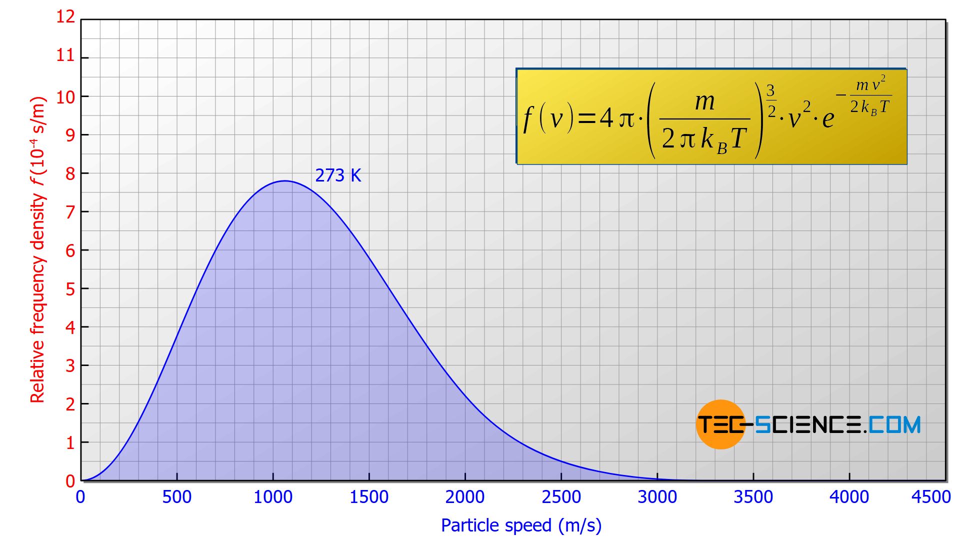
In equation (\ref{p}), m denotes the mass of a particle (not the total mass of the gas!). For a helium particle as assumed for the graph above, the mass is m = 6.6465⋅10-27 kg. The constant kB is the so-called Boltzmann constant with a value of kB = 1.38065⋅10-23 J/kg. The temperature T must be expressed in the unit Kelvin! For the considered case T=273 K (0 °C) applies. Note that the speed distribution is independent of the gas pressure!
The distribution of the molecular speeds for an ideal gas is independent of the gas pressure!
The article Determination of the speed distribution in a gas deals with the experimental determination of such a speed distribution in more detail. For ideal gases, this speed distribution can also be derived mathematically as shown in the article Derivation of the Maxwell-Boltzmann distribution function. In this article, however, the speed distribution will only be explained and interpreted in more detail.
Interpretation of the Maxwell-Boltzmann distribution function
The Maxwell-Boltzmann distribution describes the frequency with which certain molecular speeds occur in an ideal gas. In principle, however, it is not possible to assign a specific number of molecules to a specific speed. One will never find a single molecule with a specified velocity down to the “last” decimal place. One can only assign speed intervals to a concrete number of particles, i.e. the number of particles whose speeds lie within a certain range (e.g. between 1300 m/s and 1600 m/s).
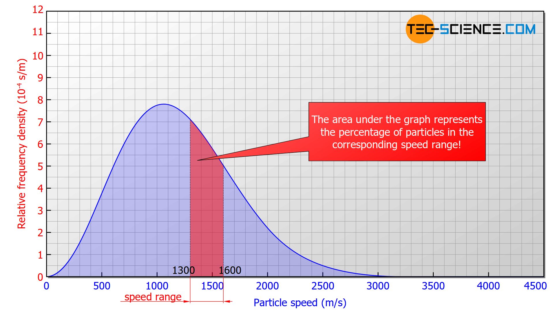
Therefore one chooses a graph in which the area under the curve corresponds to the percentage share of the particles whose speed lies within the considered interval! Therefore one does not speak of the frequency but of the frequency density (“frequency with respect to the speed interval”). As it is not an absolute frequency (i.e. not a concrete number of molecules) but a percentage, it is referred to as the relative frequency density.
The area under the Maxwell-Boltzmann distribution function corresponds to the percentage of particles whose speeds lie within the considered interval!
More detailed information on the derivation and interpretation of such a graph can be found in the article Determination of the speed distribution in a gas!
If, for example, there is an area of 0.2 in the range between 1300 m/s and 1600 m/s (see figure above), this means that 20 % of the particles have a speed within this range. If one randomly selects 100 particles in this gas, then 20 particles would be among them whose speeds lie within this interval. The probability of catching a particle whose speed lies within this interval would thus be 20 %. This example shows that the relative frequency density can also be interpreted as the probability density.
The relative frequency density can also be understood as probability density, i.e. the probability to encounter a particle within a certain speed range!
With this interpretation it also becomes clear that if only a certain speed is considered, the area under the curve becomes zero. Thus, the probability of finding a particle with exactly this velocity is also zero! This means that there is no particle with an exactly given speed.
Influence of temperature on the speed distribution
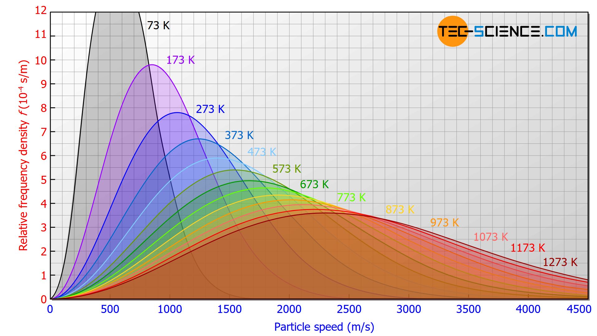
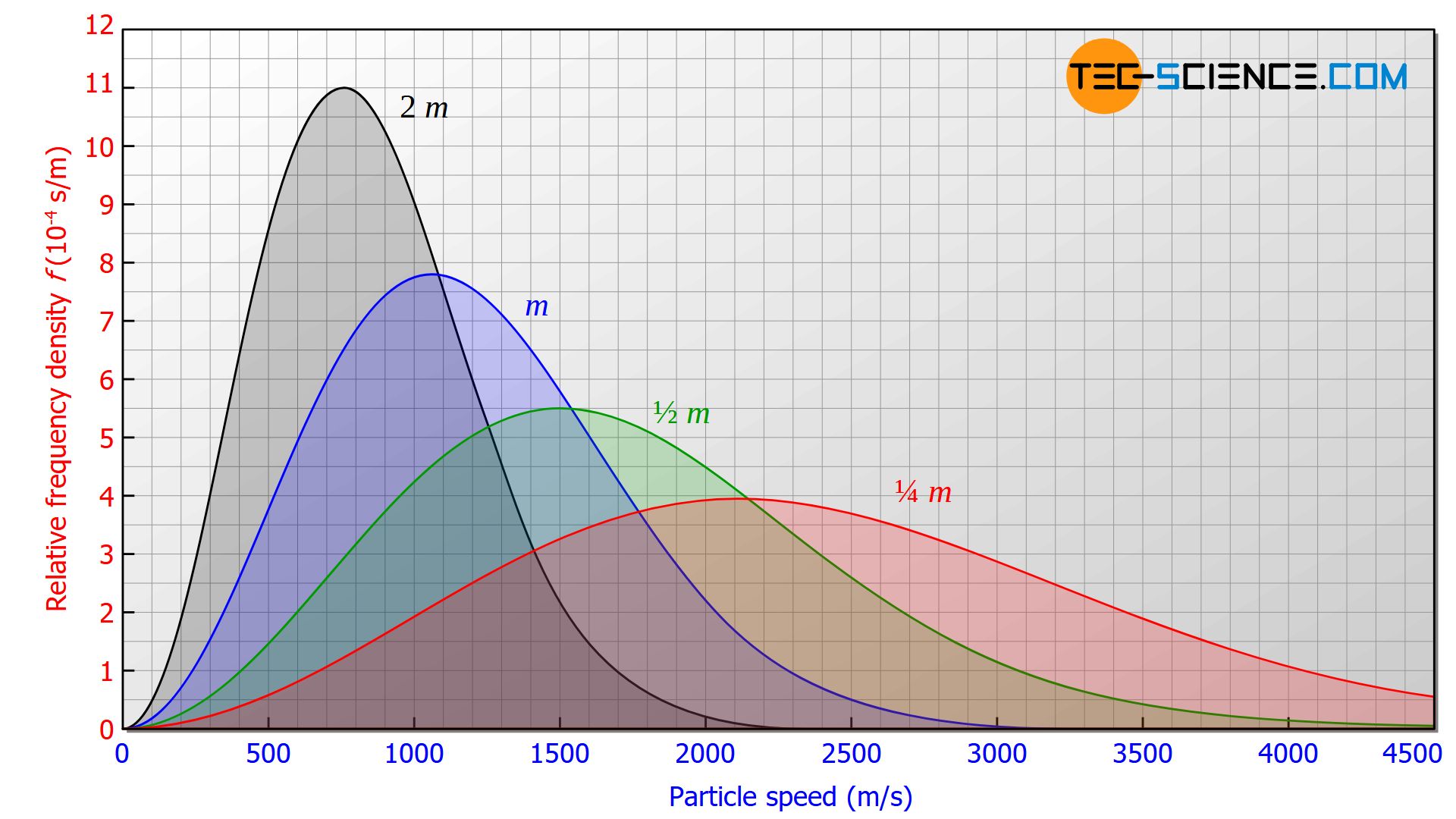
The effects of ever higher temperatures on the Maxwell-Boltzmann distribution are shown in the figure below. As the temperature rises, the curve maximum shifts to higher and higher speeds. The curves are stretched in length and squeezed in height. This results in a broader speed distribution for high temperatures, with higher speed proportions.
With increasing temperatures, the curve maximum shifts to higher and higher speeds!
However, all curves are basically “open to the right”, i.e. even at very low temperatures, there are a few particles with very high speeds!
Even at very low temperatures, there are gas molecules that have very high speeds!
If this statement is transferred qualitatively to liquids, then it can also be used to explain why liquids gradually enter the gas phase, i.e. evaporate, even far below the boiling point. Even at such low temperatures, there are always particles that have a sufficiently high velocity and thus kinetic energy to escape the attraction forces within the liquid phase. They practically break away from the binding forces and thus escape from the liquid. The liquid gradually becomes less until the molecules are completely in the gas phase. Since according to the speed distribution the number of particles that have such a sufficiently high velocity is relatively small, such an evaporation process takes a relatively long time compared to the vaporisation process. Further information can be found in the article Evaporation of liquids.
Characteristic speeds
To characterize the speed distribution, different speeds are introduced, which are explained in more detail in the following.
Most probable speed
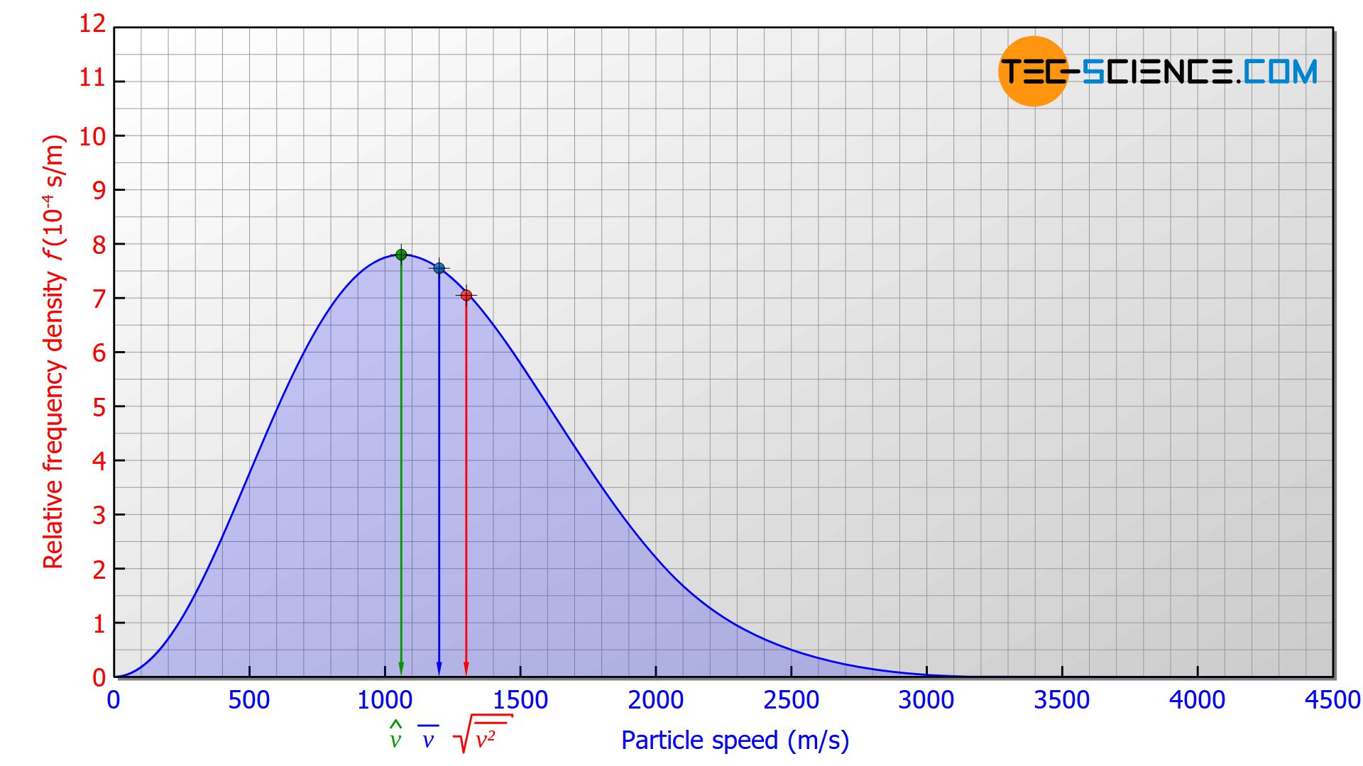
If a particle is randomly picked out of an ideal gas, it is most likely to be in the speed range with the highest proportion. This corresponds to the maximum of the speed distribution and is referred to as the most probable speed \(\hat{v}\).
Mathematically, this most likely speed can be determined by setting the first derivative of the Maxwell-Boltzmann distribution (\ref{p}) to zero [df(v)/dv=0]. The result is the following formula for determining the most probable speed:
\begin{align}
\label{w}
&\boxed{ \hat{v} = \sqrt{\frac{2 k_B T}{m}} } ~~~\text{most probable speed}\\[5px]
\end{align}
The most probable speed is not only a function of temperature but also depends on the mass of the particles. Thus, the most probable speed cannot be deduced directly from the temperature of a gas. Two different gases (whose particles have different masses) therefore have different most probable speeds despite the same temperature (see figure below). For heavier gas molecules, the most probable speeds will be lower than for lighter molecules.
Arithmetic mean speed
Another characteristic speed of the Maxwell-Boltzmann distribution is the arithmetic mean speed \(\overline{v}\) of a particle (also called average speed or just mean speed).
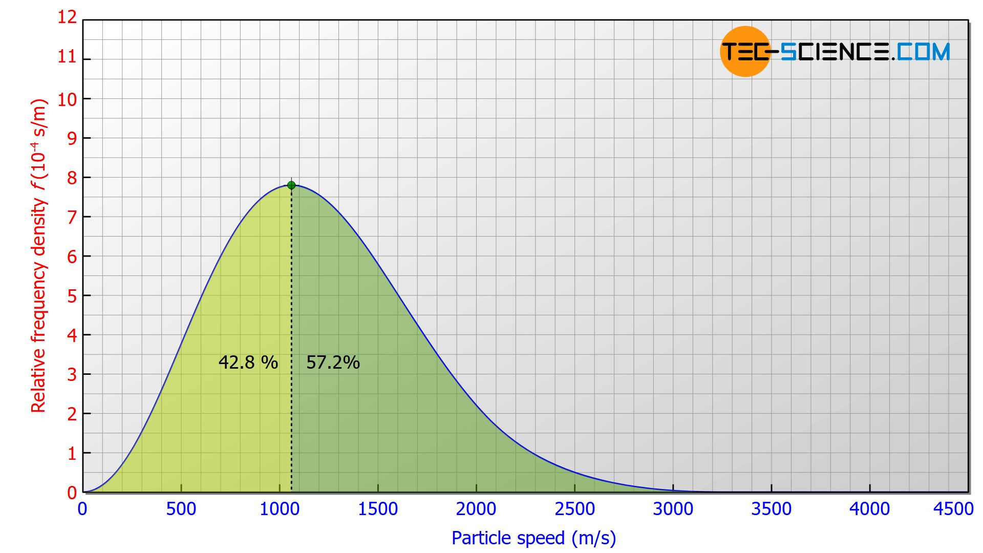
Compared to the most probable speed, the mean speed will be higher, since the number of particles with a higher speed than the most probable is also higher. This becomes clear when the area to the right and to the left of the maximum is compared. 42.8 % of the particles have a velocity below the most probable speed and 57.2 % have a velocity above the most probable speed.
The average speed is obtained by summing up the speeds of the particles and then dividing the sum by the number of particles. Mathematically, this can be calculated by solving the integral ∫v⋅f(v) dv within the entire speed range from 0 to ∞:
\begin{align}
&\overline{v} = \frac{v_1+v_2+v_3+…+v_N}{N} = \frac{\sum_{i=1}^{N}{v_i}}{N} = \int_0^\infty \! v~f(v) \, \mathrm{d}v \\[5px]
\label{a}
&\boxed{ \overline{v} = \sqrt{\frac{8 k_B T}{\pi m}} } ~~~\text{mean speed} \\[5px]
\end{align}
At this point it can be seen again that the temperature is not a direct measure of the average particle speed. The particles in a gas with four times the particle mass are on average only half as fast, even with the same temperature.
To get an impression of the order of magnitude of the mean speed in gases, nitrogen molecules N2 are considered, which make up the majority of the air with 78 %. With a particle mass of 4.65⋅10-27 kg, the nitrogen molecules have a mean speed of about 470 m/s at 273 K. Note that the average speed of the nitrogen molecules in the air is thus greater than the speed of sound! In contrast to sound, a nitrogen molecule does not travel several meters or even kilometers in a certain direction. It will permanently collide with other air particles and constantly change direction. Such a distance without a collision is usually only a few nanometers and is called the mean free path!
Root-mean-square speed
However, neither the most probable speed nor the average speed is relevant for determining the kinetic energy of a molecule. This is due to the quadratic influence of velocity on kinetic energy. Higher speeds have a disproportionately strong effect on kinetic energy. Thus, a speed twice as high does not mean a kinetic energy twice as high but four times as high. Higher speeds influence the average kinetic energy more than lower speeds.
Therefore, the mean speed must not be used to characterize the kinetic energy of a particle. Rather, the arithmetic mean of the speed squares must be taken as a basis. In order to obtain the dimension of a speed, the square root of this mean value must be calculated. This speed is then referred to as the root-mean-square speed vrms:
\begin{align}
&\boxed{v_{rms} = \sqrt{\overline{v^2}}} \\[5px]
\end{align}
For the calculation of the root-mean-square speed from the Maxwell-Boltzmann function, the square root of the integral ∫v²⋅f(v) dv has to be calculated within the range between 0 and ∞:
\begin{align}
& v_{rms} = \sqrt{\overline{v^2}} = \sqrt{\frac{v_1^2+v_2^2+v_3^2+…+v_N^2}{N}} = \sqrt{\frac{\sum_{i=1}^{N}{v_i^2}}{N}} = \sqrt{\int_0^\infty \! v^2~f(v) \, \mathrm{d}v }\\[5px]
\label{q}
&\boxed{v_{rms} = \sqrt{\frac{3 k_B T}{m}} } ~~~\text{root-mean-square speed} \\[5px]
\end{align}
It now becomes apparent that the root-mean-square speed is decisive for the average kinetic energy of a particle:
\begin{align}
\overline{W_{kin}} &= \tfrac{W_{kin,1}+W_{kin,2}+W_{kin,3} + … + W_{kin,N}}{N} = {\tfrac{\frac{1}{2}m\cdot v_1^2+\frac{1}{2}m\cdot v_2^2+\frac{1}{2}m\cdot v_3^2+…+\frac{1}{2}m\cdot v_N^2}{N}} \\[5px]
&= \frac{1}{2}m\cdot \underbrace{{\tfrac{v_1^2+v_2^2+v_3^2+…+v_N^2}{N}}}_{v_{rms}^2} = \frac{1}{2} m \cdot v_{rms}^2 \\[5px]
\end{align}
\begin{align}
\label{e}
\boxed{\overline{W_{kin}} = \frac{1}{2} m \cdot v_{rms}^2} \\[5px]
\end{align}
Relationship between the different speeds
The average speed of the particles \(\overline{v}\) is always greater than the most probable speed \(\hat{v}\), and the root-mean-square speed \(v_{rms}\) is greater than the average speed. The different speeds are in a constant ratio to each other, independent of temperature or mass. For the ratio of average speed \(\overline{v}\) to most probable speed \(\hat{v}\) applies:
\begin{align}
\frac{\overline{v}}{\hat{v}}= \frac{\sqrt{\frac{8 k_B T}{\pi m}} }{
\sqrt{\frac{2 k_B T}{m}} } = \sqrt{\frac{4}{\pi}} = 1,128\\[5px]
\end{align}
For the ratio of root-mean-square speed \(v_{rms}\) to average speed \(\overline{v}\) a value of 1.085 is obtained:
\begin{align}
\frac{v_{rms}}{\overline{v}}= \frac{\sqrt{\frac{3 k_B T}{m}}}{\sqrt{\frac{8 k_B T}{\pi m}}} = \sqrt{\frac{3\pi}{8}} = 1,085\\[5px]
\end{align}
The average speed is therefore always 12,8 % higher than the most probable speed and the root-mean-square speed is always 8,5 % higher than the average speed.
Relationship between temperature and kinetic energy
The different speeds (the most probable speed, the average speed and the root-mean-square speed) depend not only on the temperature but also on the particle mass. The frequently heard statement that the temperature is a measure for the speed of the particles is strictly speaking not correct.
For example, such a statement does not apply if two different types of gas are considered. Even at temperatures of 473 K (200 °C) the particle speeds of argon are more than half lower compared to the particle speeds of helium at 273 K (0 °C), because argon has an atomic mass about 40 times larger than helium.
Rather, the statement about the temperature aims at the average kinetic energy of the molecules. This becomes clear when the formula for the root-mean-square speed (\ref{q}) is used in equation for the average kinetic energy (\ref{e}):
\begin{align}
&\overline{W_{kin}} = \frac{1}{2} m \cdot v_{rms}^2 = \frac{1}{2} m \cdot \frac{3 k_B T}{m} \\[5px]
\label{wkint}
&\boxed{\overline{W_{kin}}=\frac{3}{2}~k_B~T } \\[5px]
\end{align}
The average kinetic energy of a particle is directly connected to the temperature and independent of the particle mass! Thus the temperature is directly a measure for the average kinetic energy of the gas particles of an ideal gas. This equation is remarkable because it combines a macroscopically measurable quantity (in the form of temperature) with a microscopic quantity (in the form of the kinetic energy of a particle)!
The temperature of an ideal gas is directly a measure of the average kinetic energy of the particles!
Equation (\ref{wkint}) was already derived in the article Pressure and temperature by kinematic and statistical considerations. It is no coincidence at this point that the Maxwell-Boltzmann distribution comes to the same conclusion. After all, the derivation of the Maxwell-Boltzmann distribution function is based on the assumption that the mean kinetic energy of a particle is linked to the temperature according to the equation (\ref{wkint})!
Maxwell-Boltzmann kinetic energy distribution
Since a certain kinetic energy can be assigned to each speed, the speed distribution can also be converted into an energy distribution. Instead of the distribution function f(v) for the speed, a distribution function for the kinetic energy g(W) is obtained.
As already explained, the (relative) frequency with which a speed exists within the limits between \(v_1\) and \(v_2\) results from the integral of the distribution function f(v):
\begin{align}
& \text{Frequency} = \int_{v_1}^{v_2} \! f(v) \, \mathrm{d}v \\[5px]
\end{align}
If the speeds v1 and v2 are converted into the respective kinetic energies W1 and W2, then a distribution function of the energy g(Wkin) within these limits must lead to the same frequency:
\begin{align}
& \text{Frequency} = \int_{W_{1}}^{W_{2}} \! g(W) \, \mathrm{d}W \\[5px]
\end{align}
If both equations are equated, then the following relationship between the two distribution functions is obtained:
\begin{align}
\int_{W_{1}}^{W_{2}} \! g(W) \, \mathrm{d}W &= \int_{v_1}^{v_2} \! f(v) \, \mathrm{d}v \\[5px]
g(W) \text{d}W &=f(v) ~ \text{d}v \\[5px]
g(W) &= f(v) ~ \frac{\text{d}v}{\text{d}W} \\[5px]
g(W) &= f(v) ~ \dfrac{1}{\frac{\text{d}W}{\text{d}v}} \\[5px]
\end{align}
The expression dW/dv contained in the denominator corresponds mathematically to the speed derivative of the kinetic energy:
\begin{align}
& \frac{\text{d}W(v)}{\text{d}v} = \frac{\text{d}(\tfrac{1}{2}mv^2)}{\text{d}v} = mv \\[5px]
\end{align}
Thus the distribution function of the kinetic energy g(W) can be determined from the distribution function of the speed f(v):
\begin{align}
&g(W) = f(v) ~ \dfrac{1}{\frac{\text{d}W}{\text{d}v}} = f(v) ~ \dfrac{1}{mv} \\[5px]
&\boxed{g(W) = f(v) ~ \dfrac{1}{mv} } \\[5px]
\end{align}
If the speed distribution f(v) is used at this point and the terms are transformed and summarized in such a way that only the kinetic energies can be found in them, then the following distribution function of the kinetic energy becomes apparent:
\begin{align}
\require{cancel}
g(W) &= \left( \sqrt{\frac{m}{2 \pi k_B T}} \right)^{3} 4 \pi v^2 \cdot \exp{\left(- \frac{\color{red}{m v^2}}{\color{red}{2} k_B T} \right)} ~ \dfrac{1}{mv} \\[5px]
& = \left( \sqrt{\frac{m}{2 \pi k_B T}} \right)^{3} 4 \pi \frac{v^\bcancel{2}}{m\bcancel{v}} \cdot \exp{\left(- \frac{\color{red}{\tfrac{1}{2}m v^2}}{k_B T} \right)} \\[5px]
& = \sqrt{\left( \frac{m}{2 \pi k_B T} \right)^{3}} \cdot 4 \pi \frac{v}{m} \cdot \exp{\left(- \frac{\color{red}{\tfrac{1}{2}m v^2}}{k_B T} \right)} \\[5px]
& = \sqrt{\left( \frac{m}{2 \pi k_B T} \right)^{3}} \cdot \sqrt{\left(4 \pi \frac{v}{m} \right)^2} \cdot \exp{\left(- \frac{\color{red}{\tfrac{1}{2}m v^2}}{k_B T} \right)} \\[5px]
& = \sqrt{\left( \frac{m}{2 \pi k_B T} \right)^{3} \cdot \left(4 \pi \frac{v}{m} \right)^2} \cdot \exp{\left(- \frac{\color{red}{\tfrac{1}{2}m v^2}}{k_B T} \right)} \\[5px]
& = \sqrt{ \frac{m^\bcancel{3}}{8 \pi^3 k_B^3 T^3} \cdot 16 \pi \frac{v^2}{\bcancel{m^2}} } \cdot \exp{\left(- \frac{\color{red}{\tfrac{1}{2}m v^2}}{k_B T} \right)} \\[5px]
& = \sqrt{\frac{4}{\pi^2 k_B^3 T^3} \cdot \color{red}{\tfrac{1}{2}mv^2} } \cdot \exp{\left(- \frac{\color{red}{\tfrac{1}{2}m v^2}}{k_B T} \right)} \\[5px]
& = \frac{2}{\sqrt{\pi}}\sqrt{\left(\frac{1}{k_B T}\right)^3} \cdot \sqrt{\color{red}{\tfrac{1}{2}mv^2}} \cdot \exp{\left(- \frac{\color{red}{\tfrac{1}{2}m v^2}}{k_B T} \right)} \\[5px]
& = \frac{2}{\sqrt{\pi}}\left(\sqrt{\frac{1}{k_B T}}\right)^3 \cdot \sqrt{\color{red}{\tfrac{1}{2}mv^2}} \cdot \exp{\left(- \frac{\color{red}{\tfrac{1}{2}m v^2}}{k_B T} \right)} \\[5px]
\end{align}
The red marked terms correspond to the kinetic energy, so the distribution function can be expressed solely by the kinetic energy:
\begin{align}
&\boxed{g(W) = \frac{2}{\sqrt{\pi}}\left(\sqrt{\frac{1}{k_B T}}\right)^3 \cdot \sqrt{W} \cdot \exp{\left(- \frac{W}{k_B T} \right)}} \\[5px]
\end{align}
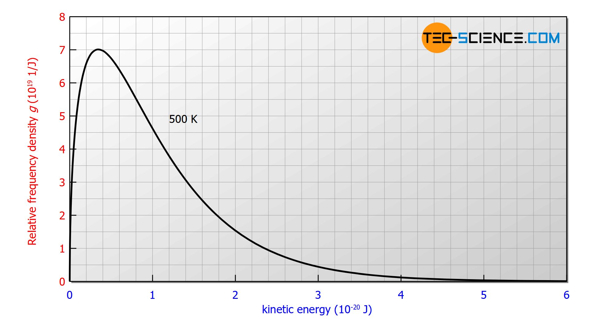
The figure below shows the distribution of the kinetic energies for a temperature of 500 K. Again, the area under the curve corresponds to the percentage of particles with kinetic energy within the corresponding limits.
In the article Derivation of the Maxwell-Boltzmann distribution function, the distribution function of the molecular speeds was derived from the barometric formula. It has already been noted that the exponential term exp(-W/kBT) describes the frequency or probability with which certain (kinetic) energies are present. This term plays a central role in statistical physics (Boltzmann statistics) and occurs whenever random distributions of energetic states are involved. For example also with Planck’s law of blackbody radiation.
The Boltzmann factor exp(-W/kBT) describes the probability with which certain energetic states are present!


")
")

