The mean free path is the average distance a particle travels without colliding with other particles!
Introduction
In the article Maxwell-Boltzmann distribution it was shown that the mean speed (average speed) of the particles of an ideal gas can be determined with the following formula:
\begin{align}
\label{v}
&\boxed{ \bar{v} = \sqrt{\frac{8 k_B T}{\pi m}} } \\[5px]
\end{align}
This formula can be used, for example, to estimate the mean speed of air particles. Since 78 % of air consists of nitrogen, the average speed of the nitrogen molecules (N2) is to be calculated. Such a nitrogen particle has a mass of 4.65⋅10-26 kg. At a temperature of 20° C (293 K) this results in a mean speed of about 470 m/s.
On average, the air particles move at supersonic speed. Due to the statistical distribution of the velocities, however, significantly higher speeds are also present. About 1 % of the molecules have a speed of more than 1000 m/s. One molecule out of one billion even reaches a speed of 2000 m/s.
If gas molecules generally have such high speeds, why not immediately perceive the smell of an open perfume bottle at the other end of a room, as one would expect at speeds of several hundred meters per second. Experience shows that it obviously takes some time for the fragrance to be noticed.
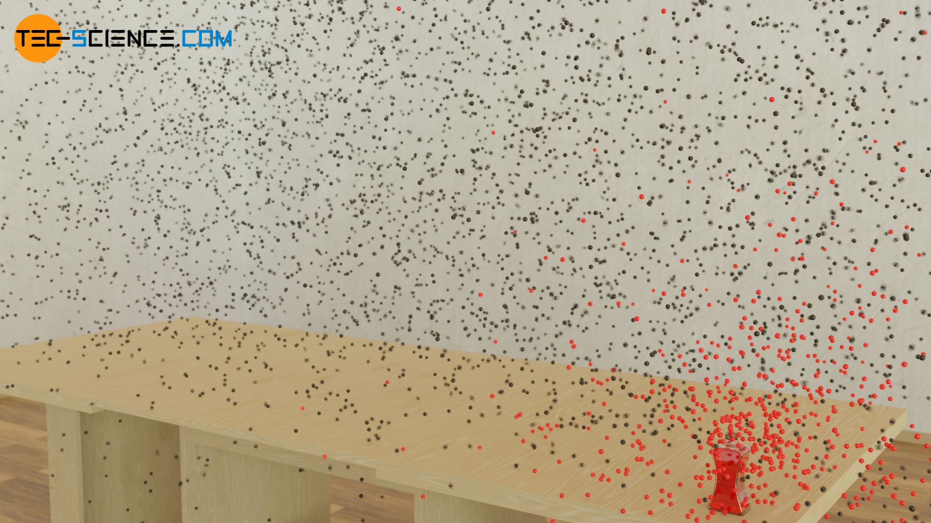
The apparent contradiction lies in the fact that the gas particles do not have a free path when moving. The molecules will permanently collide with other particles and change their direction of motion in a random way. The distance a molecule can travel on average without colliding with other molecules is called mean free path. In the present case, the relatively small mean free path of the fragrance particles prevents the perfume from being perceived immediately.
The mean free path is the average distance a particle travels without colliding with other particles!
The fact that the fragrance is nevertheless perceived relatively quickly is mainly due to air currents (convections), which carry the particles over greater distances. Note that convection is no longer a completely random motion. In this case, the molecules are moved over macroscopic distances in a certain direction.
Calculation of the mean free path
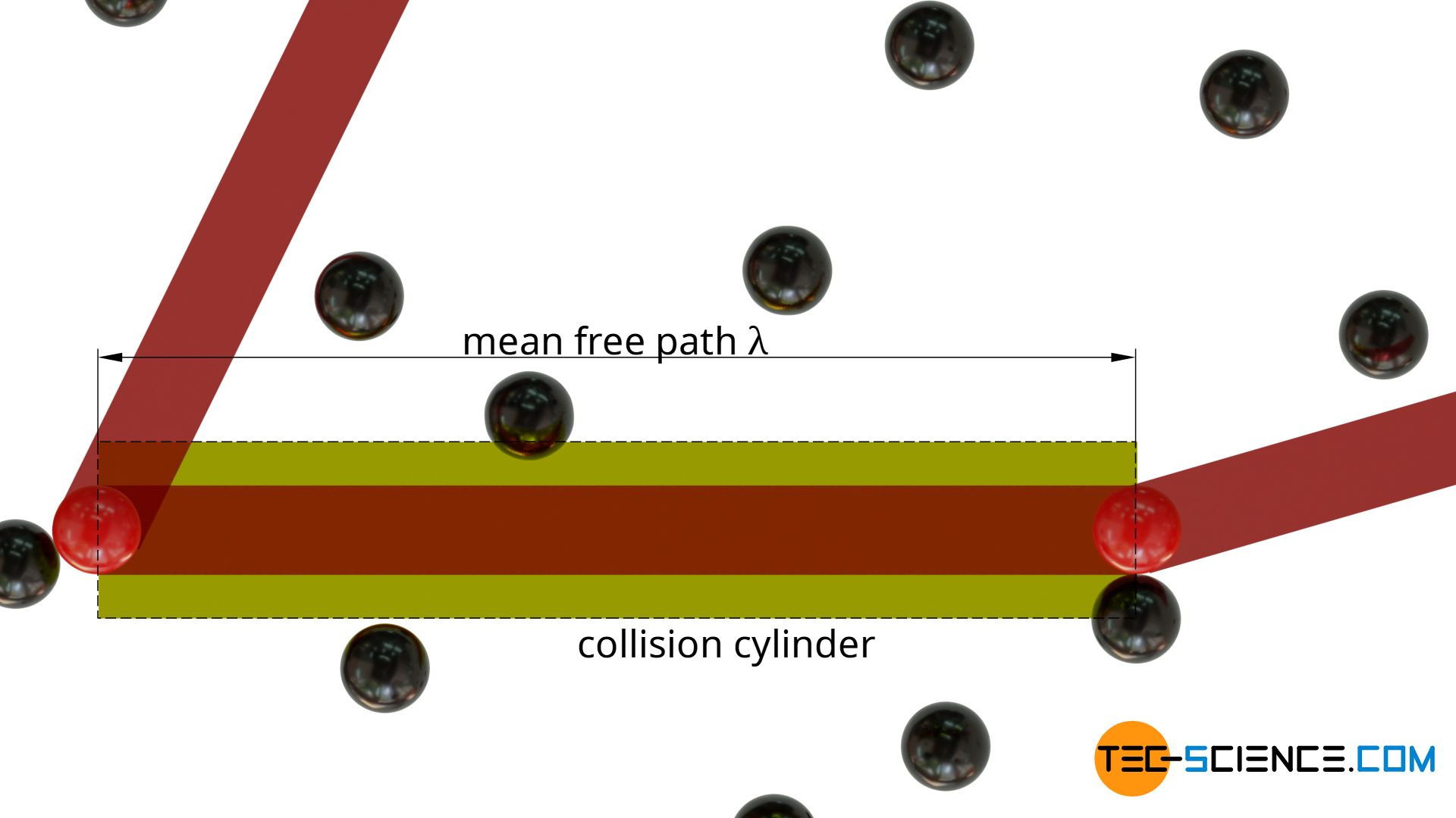
In order to determine the mean free path of a particle, a gas consisting of only one type of molecule is considered. The molecules are assumed to be spheres with a diameter d. If one now follows a particle (shown in red in the figure below), it will collide with other particles at irregular intervals (shown in black). The average distance travelled between two successive collisions corresponds to the mean free path λ.
For the sake of simplicity, all particles (with the exception of the particle followed in thought) are considered to be completely at rest. The particle traced thus moves through an “ocean” of resting particles and changes direction after each free path.
A collision between the moving particle and a stationary particle will occur when the surfaces of the spherical particles touch each other. This will be the case if the distance of the centers of gravity is smaller than twice the particle radius.
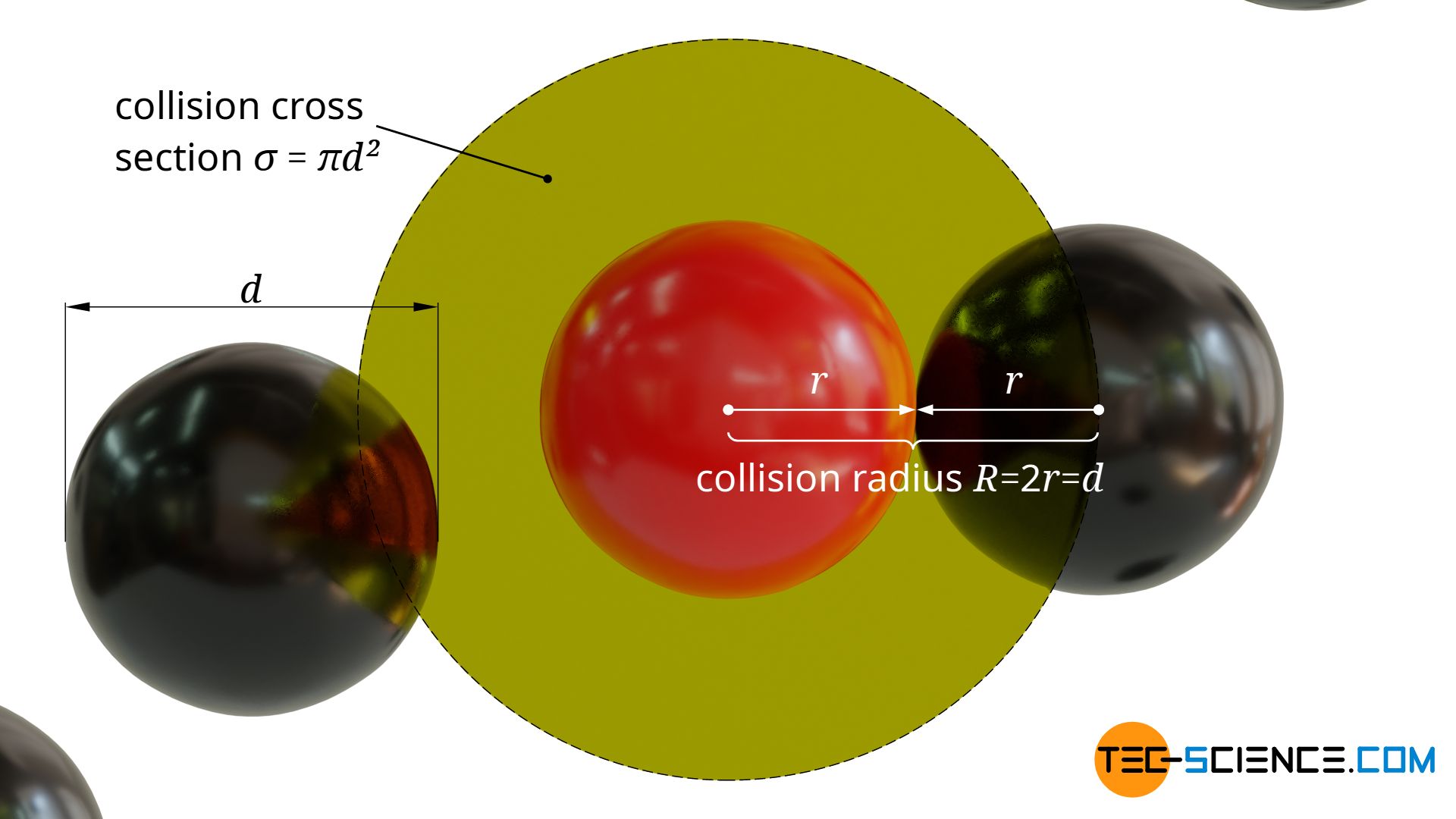
Around the center of gravity of the moving molecule a circular collision cross section σ with the radius R=2r=d can thus be defined perpendicular to the direction of motion. The center of gravity of a stationary particle must lie within this cross-sectional area in order to collide with the moving particle:
\begin{align}
&\sigma = \pi R^2 = \pi d^2 ~~~~~\text{collision cross section} \\[5px]
\end{align}
In the direction of motion, one will obtain an imaginary collision cylinder (collision volume). If the center of gravity of a particle is within this cylinder, a collision will occur. The length of the collision cylinder corresponds to the free path λ.
The (mean) volume of the collision cylinder Vc results from the product of the collision cross section σ and the length of the (mean) free path λ:
\begin{align}
& V_c = \sigma \cdot \lambda = \pi d^2 \cdot \lambda~~~~~\text{collision cylinder} \\[5px]
\end{align}
In every cylindrical collision volume Vc=σ⋅λ there is by definition just one particle, namely the particle with which the moving particle collides. Then the moving particle will change its direction and define a new collision volume, again with a “target” particle with which it will collide.
The statement that there is only one single molecule within a collision cylinder ultimately refers to the centre of gravity of the particles. In general, there will be several particles whose surface will reach into the collision volume, but only if the centre of gravity is inside this cylinder will there actually be a collision. This will only be the case for one molecule, because from then on a new collision volume will be defined, until finally a new collision will occur. This consideration of the center of gravity also makes sense insofar as the particles can still be imagined as mass points surrounded by a spherical “collision shell”. With this assumption as mass points it becomes clear that there is actually only one particle in the collision volume (see figure below).
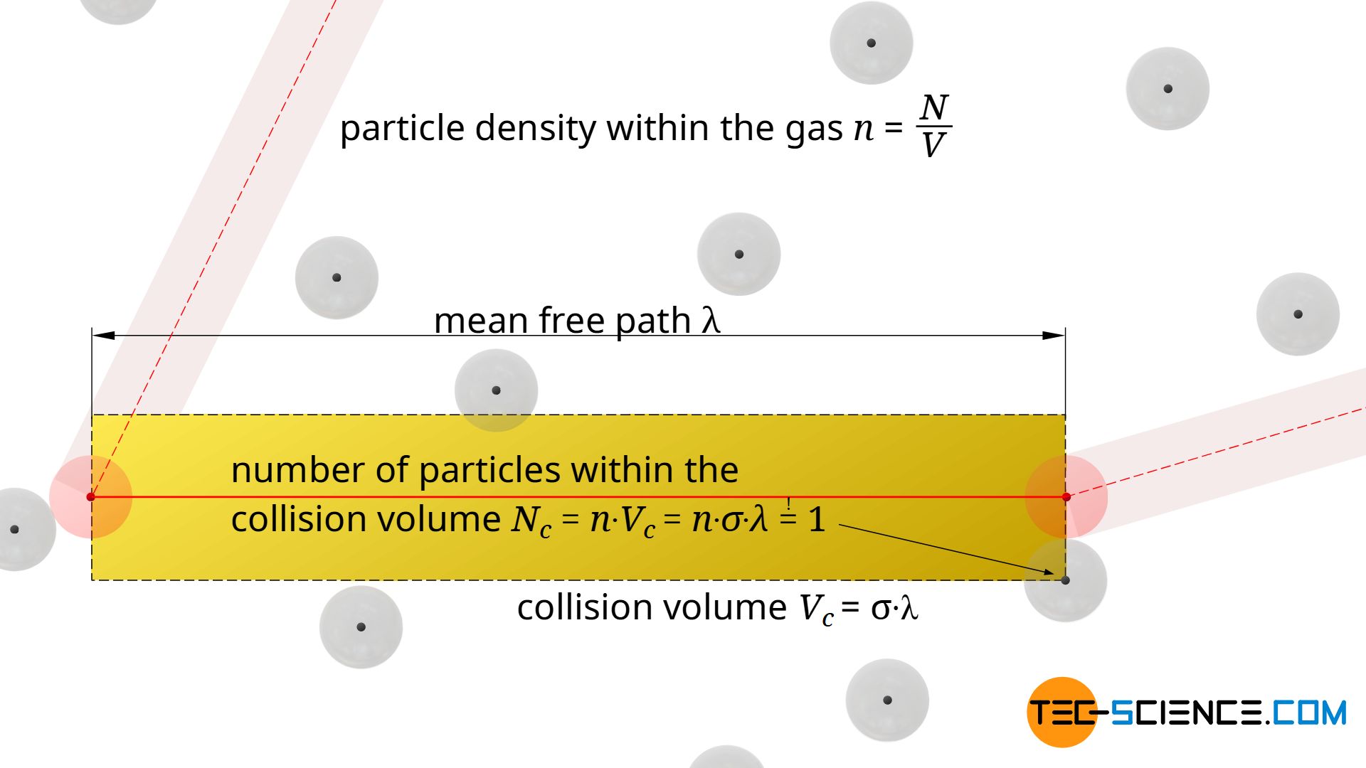
How many molecules are in a certain volume can also be determined by the particle density n in the gas. This particle density n is calculated by the quotient of the total number of particles N and the entire volume of the gas V:
\begin{align}
& n = \frac{N}{V} ~~~~~\text{particle density}\\[5px]
\end{align}
The particle density indicates the number of particles per unit volume. If one multiplies this particle density n by any volume Vc, then one obtains the average number of particles Nc inside this volume. For the collision volume, this number is of course one, so that the mean free path λ can be determined by using this condition (!):
\begin{align}
& N_c = n \cdot V_c =n \cdot 2 \pi d^2 \lambda \overset{!}{=} 1\\[5px]
& \underline{\lambda = \frac{1}{n \pi d^2}}
\end{align}
The length of the mean free path is only dependent on the particle density and the particle diameter! However, this consideration was based on stationary particles. In fact, however, the individual molecules will move relative to each other. It is to be assumed that this will then lead to increased collisions per time and therefore the mean free path will be shortened. Taking into account the Maxwell-Boltzmann speed distribution, the mean free path is then shortened by the factor 1/√2 (the derivation of this factor is shown in the last section):
\begin{align}
\label{l}
& \boxed{\lambda = \frac{1}{\sqrt{2}n \pi d^2}} ~~~~~\text{}n=\frac{N}{V}
\end{align}
For an ideal gas, the particle density n=N/V can also be expressed by the thermodynamic temperature T and the pressure p according to the ideal gas law:
\begin{align}
&pV=N k_B T ~~~~~\text{ideal gas law}\\[5px]
\label{n}
&n=\frac{N}{V}=\frac{p}{k_B T}\\[5px]
\end{align}
If equation (\ref{n}) is used in equation (\ref{l}), then the length of the mean free path can also be determined as follows:
\begin{align}
\label{lam}
& \boxed{\lambda = \frac{k_B T}{\sqrt{2} p \pi d^2}}
\end{align}
If a nitrogen molecule with a diameter of about d = 370 pm (this corresponds to a collision cross section of σ = 4.3·10-19 m²) and a temperature of T=293 K and a pressure of p=1 bar is considered, a mean free path of λ = 67 nm results. In this case, the mean free path is about 10 times less than the wavelength of visible light!
Calculation of the collision frequency
If, in addition to the length of the (mean) free path λ, the (mean) speed \(\overline{v}\) of the molecules is also known, then the (mean) time period τ between two collisions can be determined:
\begin{align}
& \text{speed } \overline{v}= \frac{\text{distance }\lambda}{\text{time } \tau} \\[5px]
\label{t}
& \boxed{\tau = \frac{\lambda}{\overline{v}}} ~~~~~\text{duration between two collisions}
\end{align}
This mean time between two collision has the meaning of a period τ, since it indicates the repetitive time intervals in which on average collisions take place. Therefore, the reciprocal of the time τ can be understood as the collision frequency f, which indicates the number of collisions per unit time. This collision frequency is often denoted by the letter Z.
\begin{align}
& Z = f = \frac{1}{\tau} \\[5px]
\label{zz}
& \boxed{Z = \frac{\overline{v}}{\lambda}} ~~~~~\text{collision frequency}
\end{align}
The number of collisions per unit time between a particle and its “target” particles is referred to as the collision frequency!
If equation (\ref{v}) for the mean speed and equation (\ref{lam}) for the mean free path are used in the formula for the collision frequency, the following formula results:
\begin{align}
&Z = \frac{\overline{v}}{\lambda}
= \frac{\sqrt{\frac{8 k_B T}{\pi m}} }{\frac{k_B T}{\sqrt{2} p \pi d^2} }
= \sqrt{\frac{8 k_B T}{\pi m}} \frac{\sqrt{2} p \pi d^2 }{k_B T}
= \sqrt{\frac{8 k_B T}{\pi m}} \sqrt{\left(\frac{\sqrt{2} p \pi d^2 }{k_B T}\right)^2} \\[5px]
&= \sqrt{\frac{8 k_B T}{\pi m} \left(\frac{\sqrt{2} p \pi d^2 }{k_B T}\right)^2}
= \sqrt{\frac{8 k_B T}{\pi m} \frac{2 p^2 \pi^2 d^4 }{k_B^2 T^2}}
= \sqrt{\frac{16 \pi p^2 d^4}{k_B T m}} \\[5px]
\label{z}
&\boxed{Z=\sqrt{\frac{16 \pi p^2 d^4}{k_B T m}} } \\[5px]
\end{align}
For the nitrogen molecule already considered at a temperature of 293 K and at a pressure of 1 bar, a collision frequency of 7·109 1/s results, i.e. within one second a single nitrogen molecule will collide on average with 7 billion other molecules!
To obtain the total number of collisions per unit volume and time, the collision frequency Z only has to be multiplied by the particle density n (“number of particles per unit volume”). It must be noted that two particles each will collide, so that a factor ½ must still be taken into account. If the particle density n is expressed by temperature and pressure according to the equation (\ref{n}), then the total number of collisions per unit volume and time is determined as follows:
\begin{align}
&z=\frac{1}{2} \cdot n \cdot Z = \frac{1}{2} \cdot \frac{p}{k_BT} \cdot \sqrt{\frac{16 \pi p^2 d^4}{k_B T m}} = \sqrt{\frac{4 \pi p^4 d^4}{k_B^3 T^3 m}} \\[5px]
&\boxed{z= \sqrt{\frac{4 \pi p^4 d^4}{k_B^3 T^3 m}} } ~~~~~\text{total number of collisions per unit volume and time}
\end{align}
For nitrogen, a total number of z = 8.7·1034 1/sm³ is obtained, i.e. 8.7·1034 collisions occur within one second in a volume of one cubic metre (a hell of a lot of collisions in a second!).
Derivation of the factor 1/√2
In this section the question shall be clarified how exactly the factor 1/√2 in the equation (\ref{lam}) for the mean free path comes about. The initial situation was the assumption that the “target” molecules of a moving molecule are all at rest.
Model conception
In analogy one can imagine a market place with many people, which one would like to cross on foot. However, all persons remain at rest for the time being. Now one starts walking straight ahead. Every time one meets a person, one randomly changes direction and then walks straight ahead again. The distance that one can walk on average without colliding with a person corresponds in a figurative sense to the mean free path.
One can determine the free path on the market place as follows. For this one has to measure the time between two collisions and on the other hand one needs the speed with which one moves. From the product of (mean) time τ0 and (mean) speed \(\overline{v}\) the (mean) free path λ results:
\begin{align}
& \lambda_0 = \overline{v} \cdot \tau_0 ~~~~~\text{mean free path for stationary “targets”}
\end{align}
Now we assume that the people on the marketplace move themselves in a chaotic way when one crosses it. The duration τ between two collisions can again be determined by a simple measurement. Although one still walks across the marketplace at the same speed, one will notice that the mean time between two collisions is shortened (τ<τ0). This also shortens the mean free path (λ<λ0):
\begin{align}
& \lambda = \overline{v} \cdot \tau ~~~~~\text{mean free path for moving “targets”}
\end{align}
The shortening of the time (or the mean free path) is ultimately due to the fact that not only the own speed determines the time interval between two collisions, but also the relative speed with which one moves towards a target. Thus, the speed of the surrounding persons is also relevant. The relative speed is basically also decisive in the case of stationary “targets”, but since these are considered to be stationary, the relative speed corresponds to the speed at which one moves oneself!
Transfering the model conception to gases
If this model conception is transferred to a gas, then the mean speed \(\overline{v}\) of a particle may not be used as the basis for the mean time between two collisions, but rather the mean relative speed \(\overline{v_{rel}}\) with which the particles approach each other on average. From statistical considerations, a relationship can be deduced between these two speeds.
For this purpose, two particles are considered which will approach each other and collide with each other. The velocity vectors of the two particles can be arranged in any way (see figure below). From the point of view of particle 1, the relative velocity at which particle 2 moves results from the difference between the velocity vectors:
\begin{align}
\label{rel1}
& \vec{v_{rel}} = \vec{v_2} – \vec{v_1} \\[5px]
\end{align}
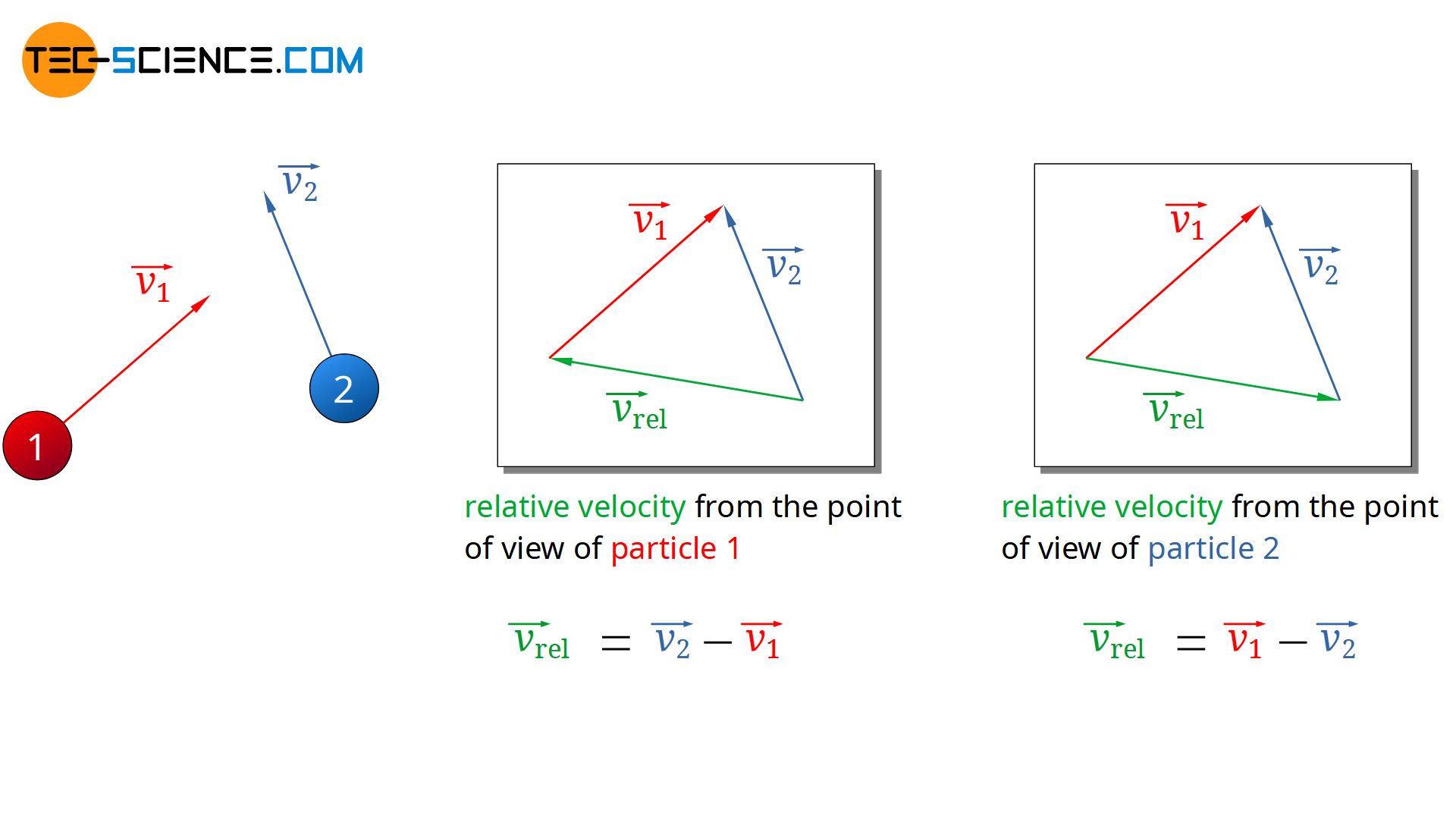
Since later anyway only the magnitude of the (mean) relative velocity vector is relevant for the (mean) free path, it would have made no difference at this point in which order the velocity vectors would have been subtracted from each other. One could have exchanged the indices in the equation above. In this way one would have described the approach of the particles from the point of view of particle 2.
Basically it makes no difference from a mathematical point of view whether you square the magnitude of a vector (v²) or whether you square the vector itself (\(\vec{v}^2\)). In both cases you get the same scalar result:
\begin{align}
\label{mat}
& v^2 = \vec{v}^2\\[5px]
\end{align}
Note: For the sake of clarity, the magnitude of a velocity ist denoted only by the symbol v without any further indication. If, on the other hand, the velocity vector \(\vec{v}\) is meant, then an arrow is explicitly placed above the symbol.
The magnitude of the relative velocity vrel (relative speed) can thus be expressed as follows by the corresponding vector \(\vec{v_{rel}}\):
\begin{align}
\label{rel2}
& v_{rel}^2 = \vec{v_{rel}}^2\\[5px]
\end{align}
If equation (\ref{rel1}) is now applied in equation (\ref{rel2}), then the following relationship results between the relative speed and the speeds of the individual particles:
\begin{align}
& v_{rel}^2= \vec{v_{rel}}^2 =\left(\vec{v_2} – \vec{v_1} \right)^2 =\vec{v_2}^2 + \vec{v_1}^2 – 2\vec{v_1}\vec{v_2} \\[5px]
\end{align}
To simplify this equation, the square of the velocity vectors can be replaced by the square of the respective speeds (see equation (\ref{mat})):
\begin{align}
& v_{rel}^2= v_2^2 + v_1^2 – 2\vec{v_1}\vec{v_2} \\[5px]
\end{align}
With this equation, only the relative speed of individual collisions can be determined so far. A statement about the mean relative speed is only possible if all potential collisions (with their respective velocity vectors) are considered and the average relative speed ist calculated:
\begin{align}
& \overline{v_{rel}^2}= \overline{v_2^2 + v_1^2 – 2\vec{v_1}\vec{v_2}} \\[5px]
\end{align}
Since the right side of the equation is the mean value of a sum, the mean value of the individual summands can be calculated instead:
\begin{align}
\label{term}
& \overline{v_{rel}^2}= \underbrace{\overline{v_2^2}}_{\text{term 1}} +
\underbrace{\overline{v_1^2}}_{\text{term 2}} –
\underbrace{\overline{2\vec{v_1}\vec{v_2}}}_{\text{term 3}} \\[5px]
\end{align}
The first term, which contains the squared speed of particle 2, does not differ on average from the second term, which contains the squared speed of particle 1. Due to the random motions, the mean speed of the two particles – or rahter all particles – is identical. It has already been mentioned that the indices could have been interchanged. This is only a question of whether the collision is observed from one particle or the other. The mean speeds v1 and v2 will thus be identical and correspond to the mean speed \(\overline{v}\) of any particle:
\begin{align}
& \overline{v_{1}^2}=\overline{v_{2}^2}=\overline{v^2} \\[5px]
\end{align}
The third term in the equation (\ref{term}) contains the scalar product of the velocity vectors. As is usual with a scalar product, the individual velocity components are multiplied by each other and then summed up. The individual components can be both negative and positive. However, since this is a completely statistical distribution of the components, positive and negative values for the scalar product are obtained to the same extent. When considering a sufficient number of particles or collisions (this is of course the case with a collision rate in the order of 1034 collisions per second and cubic meter!), the positive values of the scalar product will on average compensate the equally negative scalar products. On statistical average the third term in equation (\ref{term}) will be zero:
\begin{align}
& \overline{2\vec{v_1}\vec{v_2}} = 0 \\[5px]
\end{align}
For the mean of the squared relativ speed the following formula applies:
\begin{align}
& \overline{v_{rel}^2}= \underbrace{\overline{v_2^2}}_{\overline{v^2}} +\underbrace{\overline{v_1^2}}_{\overline{v^2}} –
\underbrace{\overline{2\vec{v_1}\vec{v_2}}}_{=0} \\[5px]
\label{vrel}
& \overline{v_{rel}^2}= 2 \cdot \overline{v^2} \\[5px]
\end{align}
According to the Maxwell-Boltzmann speed distribution, the mean of the squared speeds \(\overline{v^2}\) is in a constant ratio to the square of the mean speed (this also applies to the relative speed, because a gas does not change its temperature just because it is described from the point of view of a gas molecule):
\begin{align}
\boxed{\frac{ \sqrt{\overline{v^2}} }{\overline{v}}=\sqrt{\frac{3\pi}{8}}}\\[5px]
\end{align}
\begin{align}
\frac{ \overline{v^2} }{\overline{v}^2}&=\frac{3\pi}{8}\\[5px]
\overline{v^2} &=\frac{3\pi}{8} \cdot \overline{v}^2 \\[5px]
\end{align}
Therefore, equation (\ref{vrel}) can also be expressed by the square of the mean speed. Hence, the speeds are related by the factor √2:
\begin{align}
\require{cancel}
\overline{v_{rel}^2}&= 2 \cdot \overline{v^2} \\[5px]
\cancel{\frac{3\pi}{8}} \cdot \overline{v_{rel}}^2 &= 2 \cdot \cancel{\frac{3\pi}{8}} \cdot \overline{v}^2 \\[5px]
\end{align}
\begin{align}
&\boxed{\overline{v_{rel}}= \sqrt{2} \cdot \overline{v}} \\[5px]
\end{align}
Conclusion
The relative speed of the molecules in a gas is thus on average greater by the factor √2 than the mean speeds. The actual approach speed of two particles is therefore greater by the factor √2 than if only their own speed were taken as a basis for the approach (in principle this would correspond to the case that all other particles were at rest).
The higher speeds when taking into account the relative motions therefore shortens the time between two collisions by the factor 1/√2. Compared to the situation in which all particles are at rest, the mean free path will therefore also be smaller by the factor 1/√2! For this reason the factor 1/√2 is introduced in equation (\ref{l}).


")


