Planck’s law and Wien’s displacement law

Planck’s law describes the radiation emitted by black bodies and Wien’s displacement law the maximum of the spectral intensity of this radiation.

Blackbody radiation

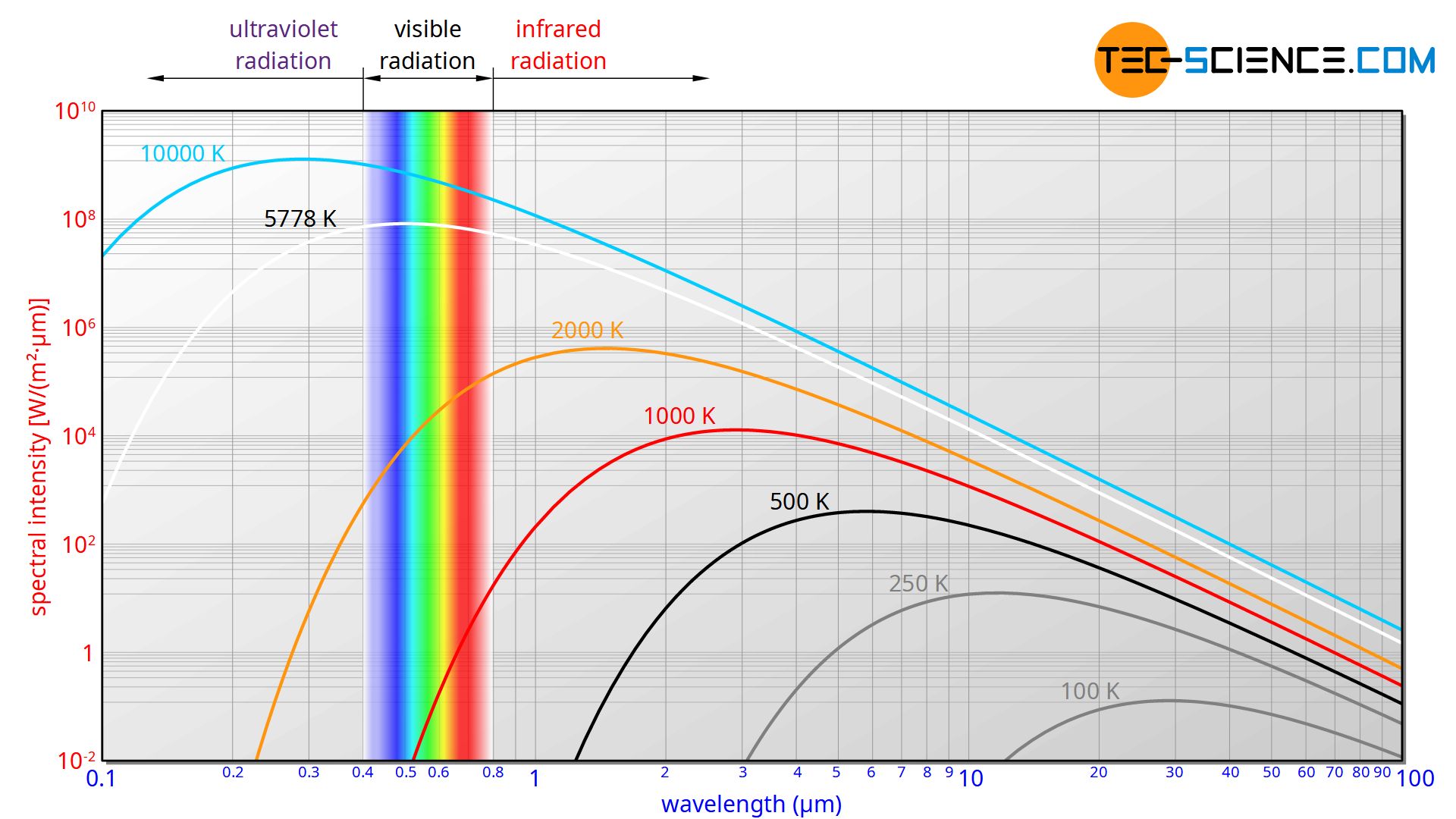
The emitted wavelength spectrum of a blackbody as shown in the figure below could not be explained for a long time. Until then, it was always assumed that energy would be distributed continuously. It was only by introducing discrete energy levels that the physicist Max Planck succeeded in describing blackbody radiation mathematically. Although he did not know how to interpret the introduction of discrete energy levels physically at first, he laid the foundation for quantum mechanics.

Planck could derive the following formula for the distribution of the spectral intensity I_s as a function of wavelength λ. This formula is also known as Planck’s law.

\begin{align}
\label{planck}
&\boxed{I_s(\lambda) = \frac{2\pi h c^2}{\lambda^5} \cdot \frac{1}{\exp\left(\dfrac{h c}{\lambda k_B T}\right)-1} } ~~~\text{Planck’s Law (wavelength form)} \\[5px]
\end{align}

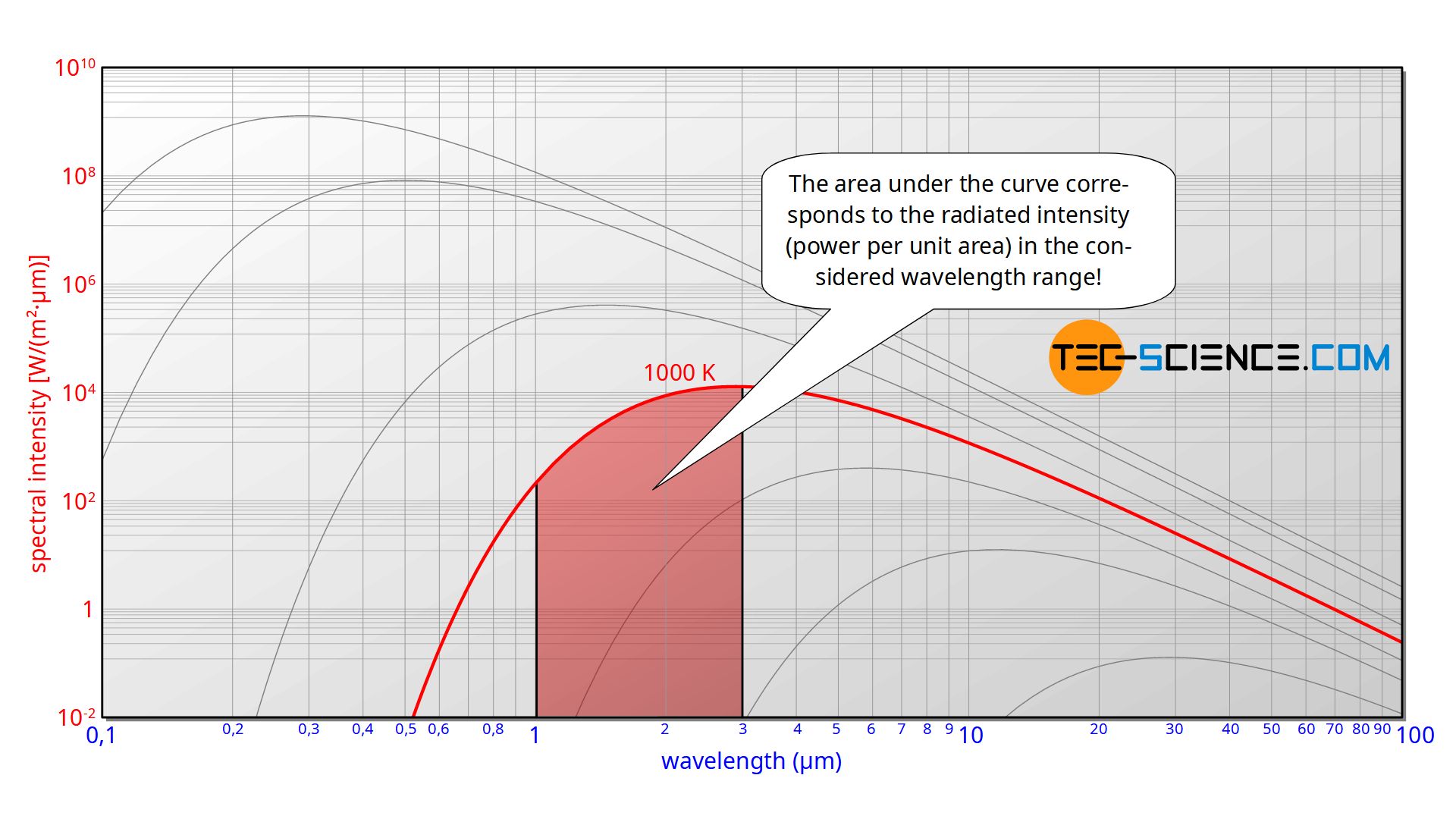
Intensity means the radiant power of the black body emitted per unit area (surface power density). If, as in this case, the intensity is related to the wavelength interval within which the power is emitted, this is called the spectral intensity. If the spectral intensity is plotted over the wavelength, then in such a diagram the area under the curve corresponds to the emitted intensity in the wavelength range under consideration.

There is a clear relationship between the wavelength λ of a radiation and its frequency f. This relationship results from the speed of propagation of the radiation, which in this case corresponds to the speed of light c (c=λ⋅f). Therefore the spectral distribution of the intensity I_s can also be expressed as a function of frequency:

\begin{align}
\label{freq}
&\boxed{I_s(f) = \frac{2\pi h f^3}{c^2} \cdot \frac{1}{\exp\left(\dfrac{h f}{k_B T}\right)-1} } ~~~\text{Planck’s law (frequency form) } \\[5px]
\end{align}

In the article Different forms of Planck’s law, the derivation of this frequency form from the wavelength form and other forms of Planck’s law are discussed in detail.

Stefan-Boltzmann law

As already mentioned, the radiated intensity results from the area under the spectral intensity distribution. Planck’s law must therefore be integrated over the entire wavelength range or frequency range. The integration is to be carried out using the frequency form (\ref{freq}):

\begin{align}
&I= \int_{0}^{\infty} I_s(f) ~ \text{d}f\\[5px]
&I= \int_{0}^{\infty} \frac{2\pi h f^3}{c^2} \cdot \frac{1}{\exp\left(\dfrac{h f}{k_B T}\right)-1} ~ \text{d}f\\[5px]
\label{her}
&I= \frac{2\pi h}{c^2} \cdot \int_{0}^{\infty} \frac{f^3}{\exp\left(\dfrac{hf }{k_B T}\right)-1} ~ \text{d}f\\[5px]
\end{align}

This integral can be solved by replacing the argument h⋅f/(k_B⋅T) of the exponential function by x (integration by substitution). Thus, the following relationships apply between the variable x and the variable f:

\begin{align}
&x := \frac{hf}{k_B T} ~~~\Rightarrow \boxed{\color{red}{f = \frac{x k_B T}{h}}} \\[5px]
&\frac{\text{d}x}{\text{d}f} = \frac{h}{k_B T} ~~~\Rightarrow \boxed{\color{blue}{\text{d}f = \frac{k_B T}{h}\text{d}x} } \\[5px]
\end{align}

If these relations are used in equation (\ref{her}), then one obtains:

\begin{align}
&I= \frac{2\pi h}{c^2} \cdot \int_{0}^{\infty} \frac{\left(\color{red}{\frac{x k_B T}{h} }\right)^3}{\exp\left(\color{red}{x} \right)-1} ~ \color{blue}{\frac{k_B T}{h}\text{d}x }\\[5px]
&I= \frac{2\pi h}{c^2} \cdot \int_{0}^{\infty} \frac{k_B^3 T^3}{h^3} \frac{x^3}{\exp\left(x \right)-1} ~ \frac{k_B T}{h}\text{d}x\\[5px]
&I= \frac{2\pi h}{c^2} \cdot \frac{k_B^3 T^3}{h^3} \cdot \frac{k_B T}{h} \cdot \int_{0}^{\infty} \frac{x^3}{\exp\left(x \right)-1} ~\text{d}x\\[5px]
&I= \frac{2\pi k_B^4}{h^3 c^2} T^4 \int_{0}^{\infty} \frac{x^3}{\exp\left(x \right)-1} ~\text{d}x\\[5px]
\end{align}

The integral ∫₀^∞ x³/(exp(x)-1) dx cannot be solved so easily in a conventional way. But a look at the mathematics formula collection shows that the result is π⁴/15. Thus the intensity of the blackbody radiation can be calculated as follows:

\begin{align}
&I= \frac{2\pi k_B^4}{h^3 c^2} T^4 \cdot \frac{\pi^4}{15}\\[5px]
&I= \underbrace{\frac{2\pi^5 k_B^4}{15 h^3 c^2}}_{\sigma} \cdot T^4 \\[5px]
&\boxed{I= \sigma \cdot T^4}~~~~~\text{and}~~~~~\boxed{\sigma = \frac{2\pi^5 k_B^4}{15 h^3 c^2}}= 5,670 \cdot 10^{-8} \frac{\text{W}}{\text{m²K}^4} \\[5px]
\end{align}

The constant quantities can be combined to a new constant, the so-called Stefan-Boltzmann constant σ (not to be confused with the Boltzmann constant k_B!). The radiated intensity of a black body is therefore only dependent on the temperature. It increases with the fourth power of the temperature. This is also called Stefan-Boltzmann law.

The Stefan-Boltzmann law states that the intensity of the blackbody radiation in thermal equilibrium is proportional to the fourth power of the temperature!

The intensity I can now be used to determine the radiant power Φ of a blackbody (also called radiant flux), i.e. its radiant energy emitted per unit time. For this the intensity I (as surface power density) has to be multiplied by the surface area A of the blackbody:

\begin{align}
&\boxed{\Phi(T,A) = \sigma \cdot A \cdot T^4} \\[5px]
\end{align}

More information on the Stefan Boltzmann Law and its derivation from thermodynamics can be found in the main article Stefan-Boltzmann law.

Real bodies: The emissivity

In practice, real objects do not radiate with the intensity of a blackbody, but have a lower radiant power. This is expressed by the unitless emissivity ε<1. The emissivity represents the radiant power of a real body compared to an ideal black body:

\begin{align}
&\boxed{I_{real}=\varepsilon \cdot \sigma \cdot T^4}\\[5px]
&\boxed{\Phi_{real} = \varepsilon \cdot \sigma \cdot A \cdot T^4} \\[5px]
\end{align}

For non-metallic surfaces, the emissivity is in many cases above 0.9. Many objects can therefore be regarded as black bodies in very good approximation with regard to the emitted radiation. This makes it relatively easy to determine the temperature of real objects with the help of a thermal imaging camera or a pyrometer, since surface properties have a rather minor influence (unless the surfaces are extremely reflective).

Wien’s displacement law

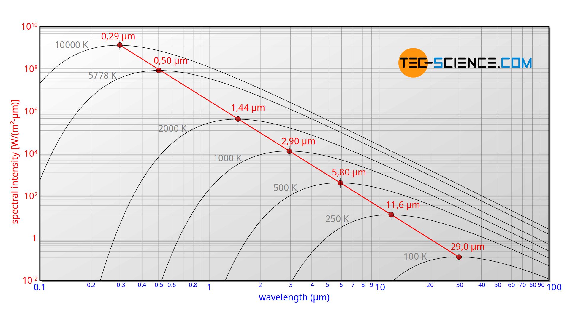
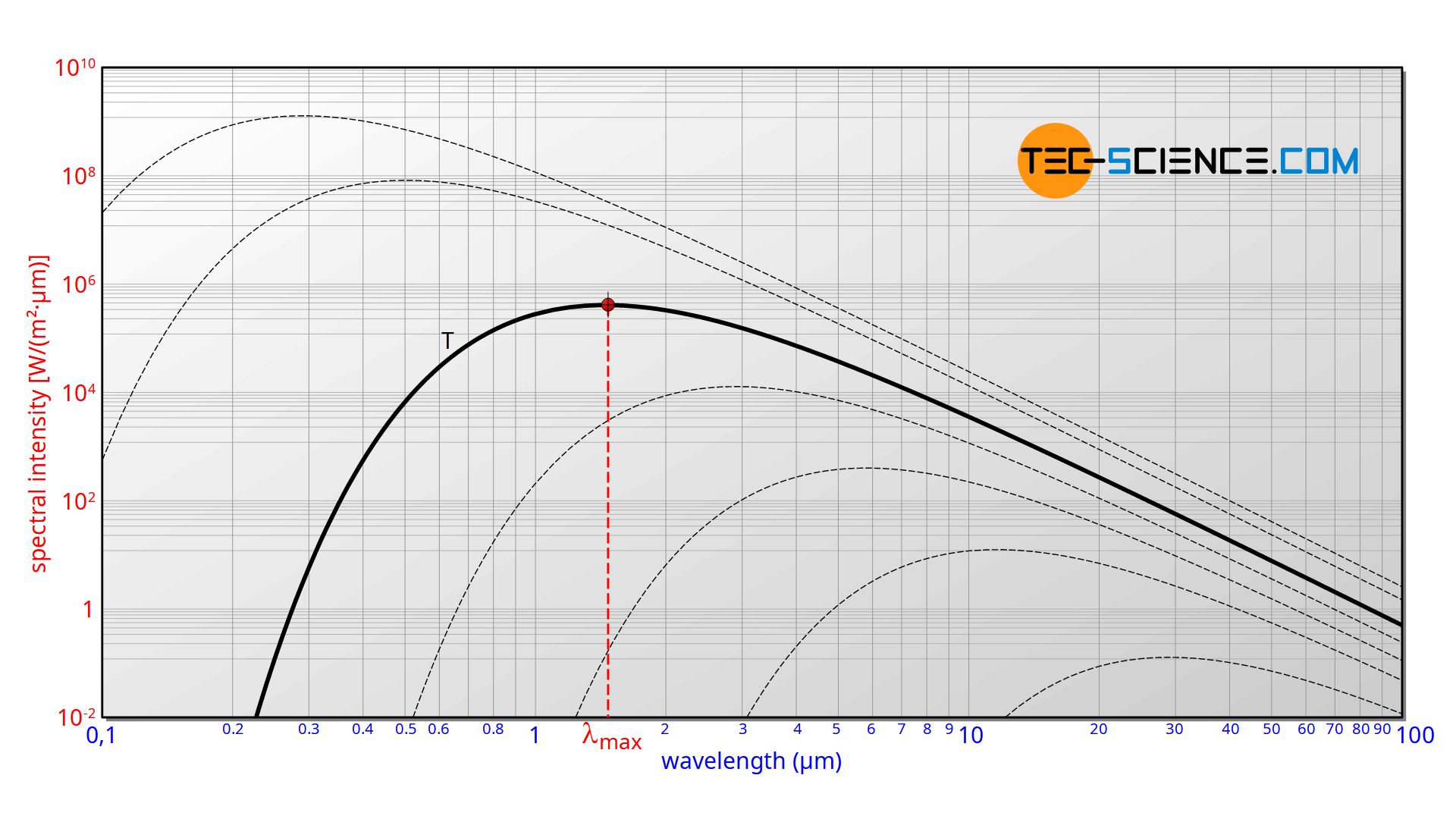
The spectral distribution as a function of temperature is now to be examined more closely. It turns out that the maximum of the curve shifts with increasing temperature to ever shorter wavelengths. The dependence of this wavelength λ_max on the temperature is given by the following equation. This equation is also known as Wien’s displacement law.

\begin{align}
&\boxed{\lambda_{max}=\frac{2897,8 \text{ µm K}}{T}}~~~\text{Wien’s displacement law} \\[5px]
\end{align}

The Wien’s displacement law can be obtained by determining the maxima of Planck’s law. For this purpose, the function (\ref{planck}) must be derived with respects to the wavelength λ. By using the product rule and setting the derivative equal to zero, one gets:

\begin{align}
\label{abl}
&\frac{\text{d}I_s(\lambda)}{\text{d}\lambda} \overset{!}{=} 0 ~~~~~\text{mit}~~~~~ I_s(\lambda) = \frac{2\pi h c^2}{\lambda^5} \cdot \frac{1}{\exp\left(\dfrac{h c}{\lambda k_B T}\right)-1} \\[5px]
\end{align}

\begin{align}
\frac{\text{d}I_s(\lambda)}{\text{d}\lambda} &= 2 \pi c^2 \left(\frac{hc}{k_B T \lambda^7} \cdot \frac{\exp\left( \frac{hc}{k_B T \lambda}\right)}{\left[\exp\left( \frac{hc}{k_B T \lambda} \right) -1\right]^2} – \frac{1}{\lambda^6} \cdot \frac{5}{\exp\left(\frac{hc}{k_B T \lambda}\right)-1} \right) \\[5px]
&= \underbrace{\frac{2 \pi c^2}{\lambda^6 \cdot \left[ \exp\left( \frac{hc}{k_B T \lambda} \right) -1 \right] }}_{>0} \underbrace{\left(\frac{hc}{k_B T \lambda} \cdot \frac{\exp\left( \frac{hc}{k_B T \lambda}\right)}{\exp\left( \frac{hc}{k_B T \lambda} \right) -1} – 5 \right)}_{=0} =0
\end{align}

This equation will only be zero if the term in the round bracket becomes zero:

\begin{align}
&\frac{hc}{k_B T \lambda} \cdot \frac{\exp\left( \frac{hc}{k_B T \lambda} \right)}{\exp\left( \frac{hc}{k_B T \lambda} \right) -1} – 5 = 0 \\[5px]
\end{align}

With the substitution given below, this equation can be simplified:

\begin{align}
\label{max}
&\boxed{x := \frac{hc}{\lambda k_B T}} ~~~\Rightarrow~~~ x \cdot \frac{\exp\left(x\right)}{\exp\left(x\right) -1} – 5 = 0 \\[5px]
\end{align}

This equation can only be solved numerically, e.g. with the Newton’s method. The result will be x = 4.9651. With this result the wavelength λ_max can be determined as a function of the temperature by solving equation (\ref{max}) for λ_max:

\begin{align}
& \lambda_{max}= \frac{hc}{x k_B T} = \frac{\tfrac{hc}{x k_B}}{T}= \frac{0,0028978 \text{ m K}}{T}= \frac{2897.8 \text{ µm K}}{T} \\[5px]
\end{align}

\begin{align}
&\boxed{\lambda_{max}=\frac{2897.8 \text{ µm K}}{T}}\\[5px]
\end{align}

The maximum of the spectral intensity can also be determined for the frequency form I_s(f). For this the function I_s(f) must be derived with respect to frequency f and setting the derivative equal to zero:

\begin{align}
&\frac{\text{d}I_s(f)}{\text{d}\lambda} \overset{!}{=} 0 ~~~\Rightarrow~~~ \boxed{f_{max} = 5.879 \cdot 10^{10} \tfrac{\text{Hz}}{\text{K}} \cdot T}
\end{align}

Remark

Note that Wien’s displacement law indicates the wavelength λ_max at which the spectral intensity has a maximum. This maximum is not to be equated with the maximum of the intensity itself or with the maximum of the radiant power! This leads for example to the fact that although the general relationship f=c/λ applies, it does not apply in this particular case f_max=c/λ_max!

This has to do with the fact that the spectral intensity is a quantity related to the wavelength. One measures the radiant power in a certain wavelength interval dλ and refers to it the radiant power. A comparison of different radiant powers is therefore only possible if the same wavelength intervals are always considered. Since the frequency is not proportional to the wavelength but reciprocally proportional, equidistant wavelength intervals do not also mean equidistant frequency intervals!

A simple example is the wavelength range between 1 and 10 µm, which is divided into intervals of 1 µm each. This results in the following equidistant series:

\begin{align}
&1-2-3-4-5-6-7-8-9-10 \\[5px]
\end{align}

The reciprocal values of this, which in the figurative sense have the meaning of the frequency as a reciprocal value of the wavelength, no longer result in an equidistant series:

\begin{align}
&\frac{1}{1}-\frac{1}{2} -\frac{1}{3} -\frac{1}{4} -\frac{1}{5} -\frac{1}{6} -\frac{1}{7} -\frac{1}{8} -\frac{1}{9} -\frac{1}{10} \\[5px]
&1-0,5-0,333-0,25-0,2-0,167-0,143-0,125-0,111-0,1 \\[5px]
\end{align}

So one cannot compare equidistant wavelength intervals with equidistant frequency intervals. Therefore a different frequency f_max than one could expect from the formula f_max=c/λ_max is obtained when using the frequency form of the spectral intensity.