Derivation of the Maxwell-Boltzmann distribution function

The Maxwell-Boltzmann distribution function of the molecular speed of ideal gases can be derived from the barometric formula.

Introduction

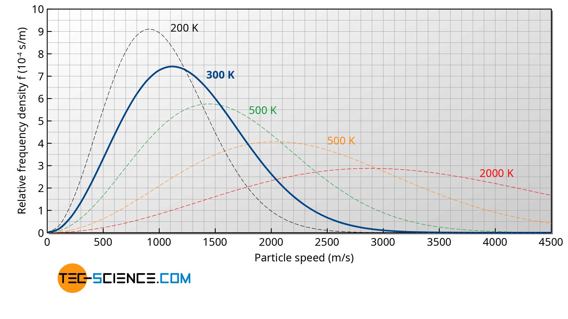
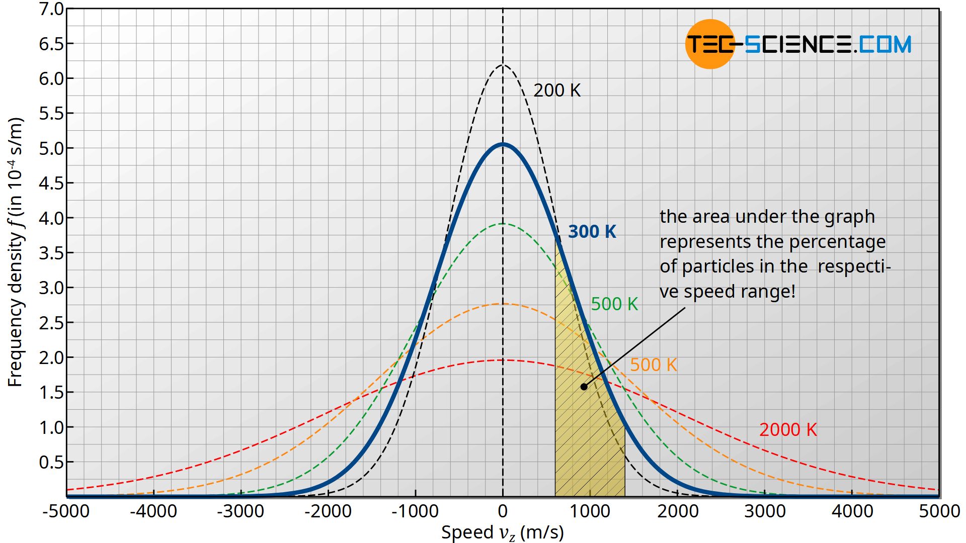
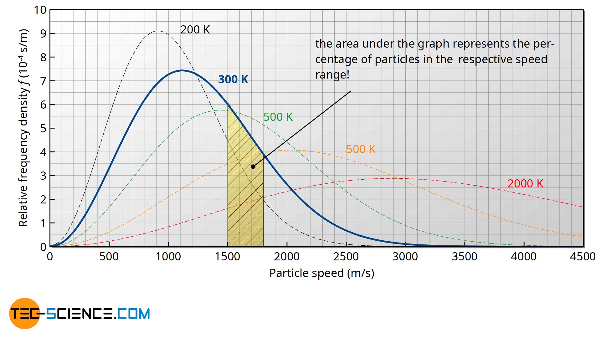
For ideal gases, the distribution function f(v) of the speeds has already been explained in detail in the article Maxwell-Boltzmann distribution. The figure below shows the distribution function for different temperatures.

\begin{align}
\label{p}
&\boxed{  f(v) = \left(  \sqrt{\frac{m}{2 \pi k_B T}}  \right)^{3}  \cdot 4 \pi v^2 \cdot \exp{\left(- \frac{m \cdot v^2}{2 k_B \cdot T} \right)} } ~~~\text{Maxwell-Boltzmann distribution function} \\[5px]
\end{align}

The purpose of this article is to derive this distribution function.

Barometric formula

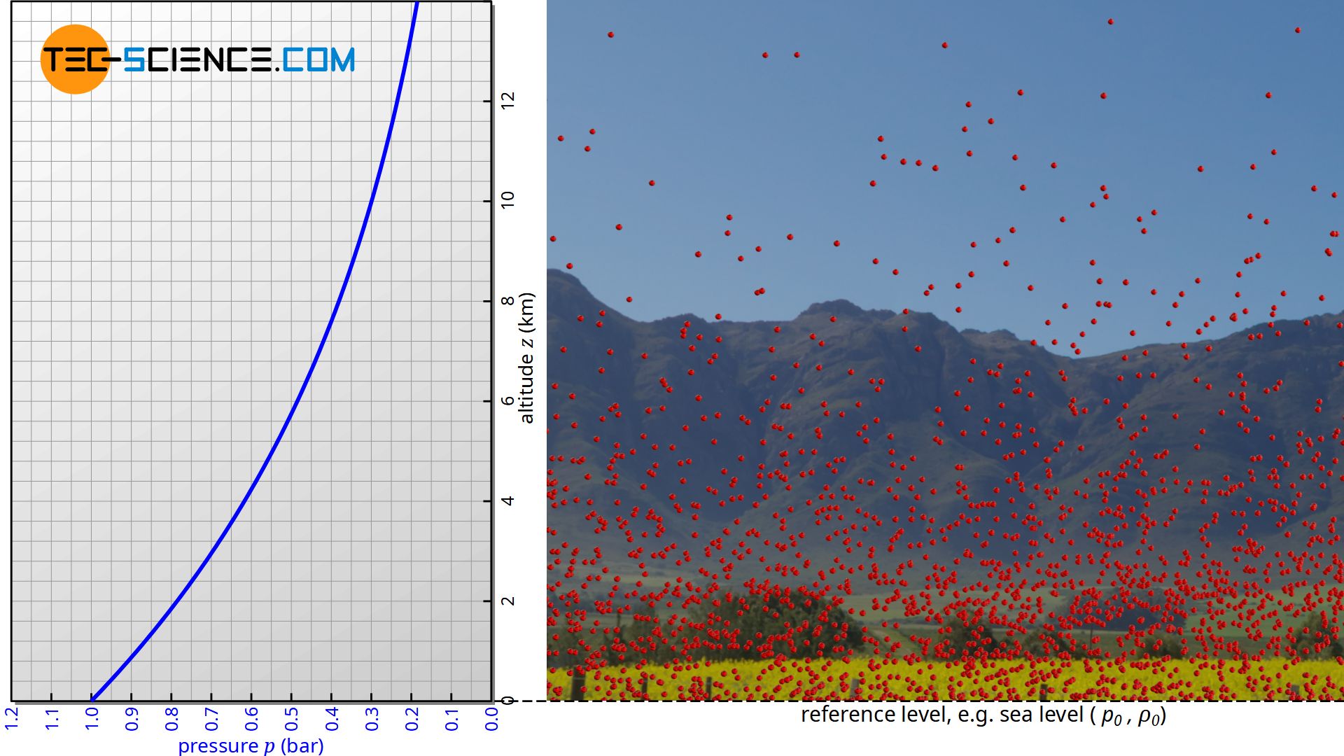
The barometric formula describes the course of atmospheric pressure p or air density ϱ as a function of altitude z above a reference level (e.g. sea level):

\begin{align}
\label{bar}
&\boxed{p(z) = p_0 \cdot \exp{\left(-\dfrac{\rho_0 g z}{p_0}\right)}} ~~~\text{barometric formula} \\[5px]
\end{align}

The barometric formula is not limited to air. It can be applied to any (ideal) gas exposed to a gravitational field. The ideal gas law shows the following relationship between the pressure p, the volume V, the number of particles N and the thermodynamic temperature T (k_B denotes the Boltzmann constant):

\begin{align}
&p V = N k_B T \\[5px]
\end{align}

The total mass of the gas m_gas (which occupies the volume V) can be determined from the product of particle mass m and number of particles N (m_gas=N⋅m). Thus the number of particles results from the quotient of gas mass and particle mass (N=m_gas/m). If this is taken into account in the equation above, then the gas density ϱ=m_gas/V can be calculated as follows:

\begin{align}
&p V = \frac{m_{gas}}{m} \cdot k_B T \\[5px]
&p = \frac{m_{gas}}{V} \cdot \frac{k_B T}{m} \\[5px]
\label{density}
&\boxed{p = \rho \cdot \frac{k_B T}{m}} ~~~\text{or}~~~\boxed{p_0 = \rho_0 \cdot \frac{k_B T}{m}} \\[5px]
\end{align}

In equation (\ref{density}), ϱ₀ denotes the gas density at the reference level and ϱ is the density associated with a pressure p. If equation (\ref{density}) is now applied in the barometric formula (\ref{bar}), then the following relationship results between the density at the reference level ϱ₀ and the density ϱ at an arbitrary height z:

\begin{align}
\require{cancel}
&p(z) = p_0 \cdot \exp{\left(-\dfrac{\rho_0 g z}{p_0}\right)} \\[5px]
&\rho(z) \cdot \bcancel{\frac{k_B T}{m}}= \rho_0 \cdot \bcancel{\frac{k_B T}{m}} \cdot \exp{\left(-\dfrac{\bcancel{\rho_0} g z}{ \bcancel{\rho_0} \cdot \frac{k_B T}{m} }\right)} \\[5px]
\label{rho}
&\rho(z)= \rho_0 \cdot \exp{\left(-\dfrac{m g z}{k_BT}\right)} \\[5px]
\end{align}

Since the mass m in equation (\ref{rho}) refers to a single molecule, the expression m⋅g⋅z can be interpreted as the potential energy W_pot) of a molecule at the height z:

\begin{align}
\label{rhoz}
&\rho(W_{pot})= \rho_0 \cdot \exp{\left(-\dfrac{W_{pot}}{k_BT}\right)} \\[5px]
\end{align}

At this point the question arises how the molecules get to their potential energy. First imagine the gas molecules at absolute zero. Due to the lack of brownian motion, all particles will be on the ground because of the influence of gravity (reference level).

Now one slowly increases the temperature by heating the gas, so that the motion of the molecules will increase. Sooner or later the molecules will collide with each other. As a result of the permanent collisions, some particles will catapult each other higher and higher. From an energetic point of view, however, this is nothing more than a supply of kinetic energy at the reference level which is subsequently converted into potential energy. We can conclude that the molecules reach their height due to their kinetic energy at the reference level (supplied by heat).

Model conception

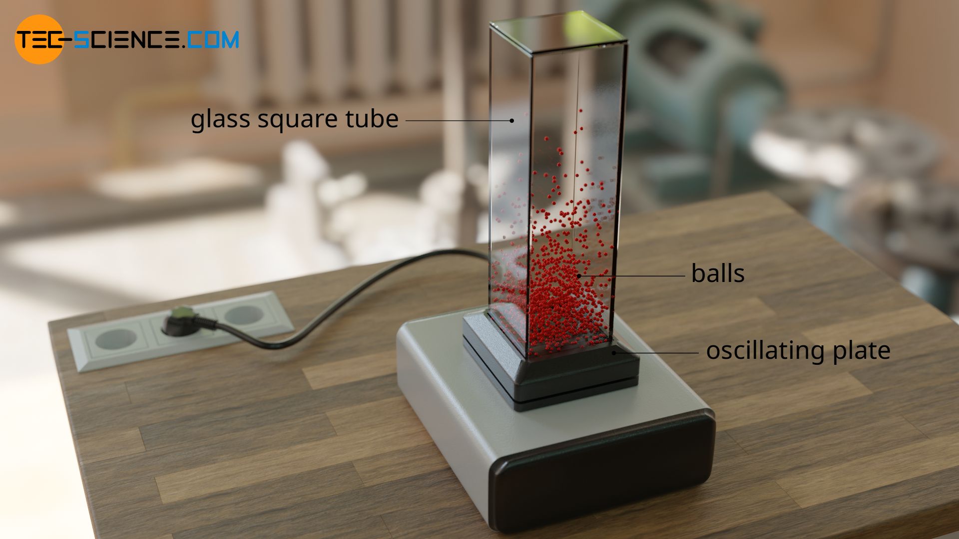
The following model can be used to describe such a behavior of the gas molecules under the influence of gravity. One puts many balls into a vertical tube, which stands on a vibrating plate. The balls will move more or less strongly depending on the strength of the vibration, just as the gas particles move more or less strongly depending on the temperature. The balls are catapulted into the air, just as the gas molecules in reality do due to their collisions.

However, one will notice that there is no uniform distribution of the balls over the altitude of the tube, as is also the case with a real gas. This is due to the fact that not all balls are supplied with the same kinetic energy at the bottom of the tube. The balls collide with each other and therefore some are slowed down and others are accelerated. If e.g. an upward flying ball is hit by a faster ball, then the kinetic energy of the pushed ball will increase. This ball will now be able to reach higher heights. If it is pushed by chance by another ball, it will be able to fly even higher. For a few balls this might happen one or two more times. Such an ideal catapult effect will only be limited to a few balls. That’s why with increasing height less and less balls are to find.

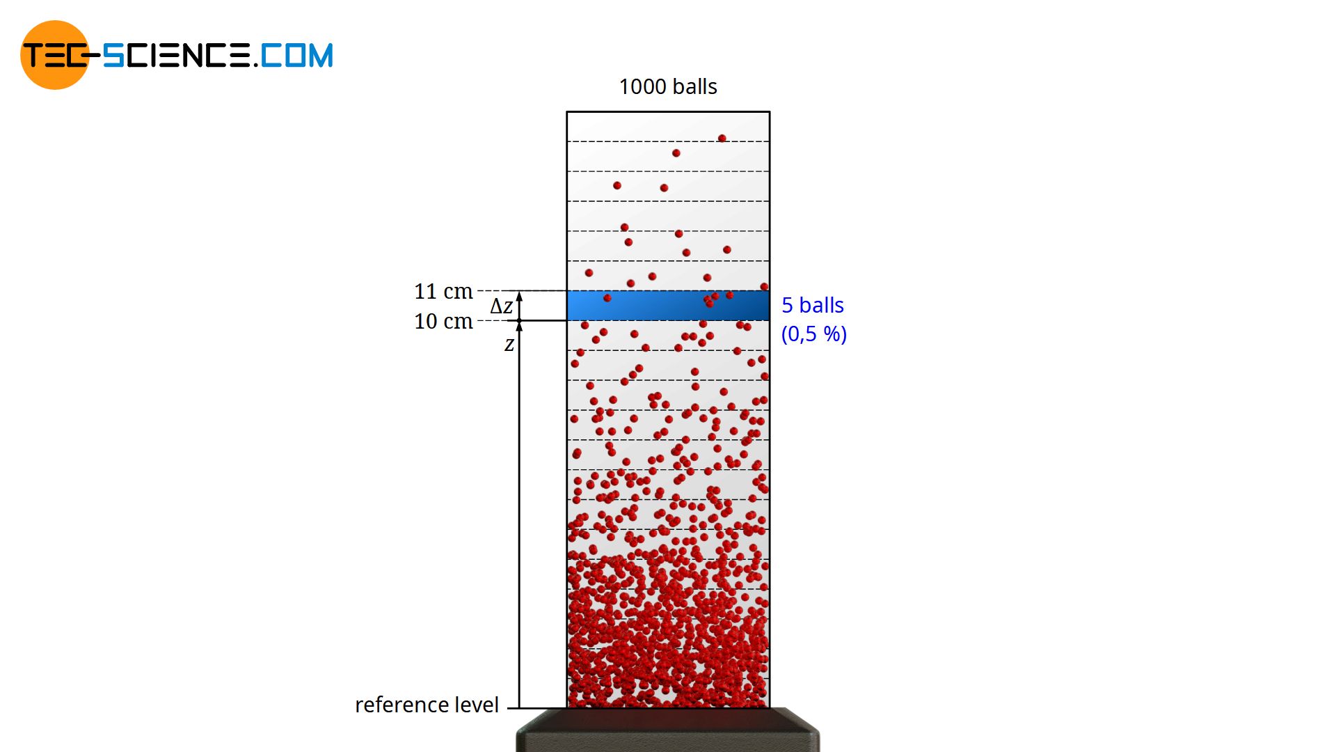
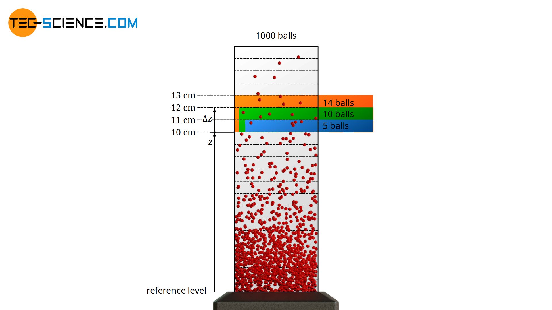
With increasing altitude, the ball density (“number of balls per unit volume”) will decrease, because it becomes more and more improbable that a ball on the ground accidentally gets such a high kinetic energy in order to reach this height (whether there are collisions with other balls on the way up or not plays no role from an energetic point of view). It should be noted that in principle it is not possible to assign a certain number of balls to a certain height. For example, you will not find a single ball at a height of exactly 10 cm, since no ball will ever reach an exact height of 10 cm up to the “last” decimal place (possibly only 10.0003 cm or 9.9998 cm).

For a concrete number of balls you have to divide the height into small intervals Δz and determine the balls occurring in them. As an example, 1000 balls are considered. Each ball has a mass of 10 g. If now at a height between 10 cm and 11 cm 5 balls are registered on statistical average, then obviously 0.5% of the total balls have a potential energy between 10 mJ and 11 mJ (the particles come to a standstill at this height and the former kinetic energy at ground level has been completely converted into potential energy). This means that 0.5 % of the balls have a kinetic energy between 10 mJ and 11 mJ at the reference level. The probability that a randomly picked ball has a kinetic energy between 10 mJ and 11 mJ is therefore also 0.5 %. The frequency with which certain energies are present can therefore also be interpreted as a probability!

The frequency with which balls are detected within a certain altitude range corresponds to the probability with which certain kinetic energy ranges are present at reference level!

Instead of the interval of Δz = 1 cm, one could have chosen an interval of Δz = 2 cm (see figure below). In this case, balls at a height between 10 cm and 12 cm are considered. The probability would be high that double the number of balls would be found. After all, we are now looking at a space that is twice as large. Strictly speaking, this proportionality only applies to (infinitely) small interval widths, since the ball density changes with height. However, this example shows that for the determination of the frequency not only the ball density at a certain height is relevant, but also the interval width that is looked at!

The ball density in combination with the height interval observed at a certain height is a measure of the frequency or probability with which the corresponding kinetic energy ranges are present at the reference level!

What does “ball density in combination with the height interval” mean in concrete terms? As already explained, for small intervals there is a proportional relationship to the number of balls contained in that interval (usually expressed in percent as a relative frequency or probability):

\begin{align}
&\text{Frequency} ~\sim \text{“interval width”} \\[5px]
\end{align}

In addition, the ball density is anyway proportional to the number of balls, because a density twice as high means by definition a number of balls twice as high (per unit volume):

\begin{align}
&\text{Frequency} ~\sim \text{“ball density”} \\[5px]
\end{align}

The frequency with which the balls are found at a certain height z and within a certain interval is thus proportional to the product of the ball density and the interval width:

\begin{align}
\label{hau}
&\boxed{\text{Frequency} ~\sim \text{“ball density”} \times \text{“interval width”} } \\[5px]
\end{align}

This model conception shows that it is possible to deduce the distribution of the kinetic energies at the reference level from the density of the balls at different heights and the interval width. The speed distribution can then be determined from this. Since only the velocity component in the z-direction is relevant for reaching a certain height, the kinetic energies refer only to the speeds related to the z-direction:

\begin{align}
\label{wpot}
&W_{pot}=W_{kin,z}=\frac{1}{2}mv_z^2 \\[5px]
\end{align}

Transfer of the model concept to gases

The ball model described above can now be transferred to gas molecules in the Earth’s gravitational field and thus to the barometric formula. The gas density decreases with increasing height because fewer and fewer particles had sufficiently high kinetic energies on the reference level to reach the corresponding height.

The mass density at a certain height is a measure of the frequency with which certain speeds are present at the reference level!

If, for this purpose, equation (\ref{wpot}) is used in equation (\ref{rhoz}), the following relationship results:

\begin{align}
&\rho(W_{pot})= \rho_0 \cdot \exp{\left(-\dfrac{W_{pot}}{k_BT}\right)} ~~~\text{and}~~~ W_{pot}=W_{kin,z}=\tfrac{1}{2}mv_z^2~~~\text{:}\\[5px]
\label{rhov}
&\boxed{\rho(v_z)= \rho_0 \cdot \exp{\left(-\dfrac{mv_z^2}{2k_BT}\right)}} \\[5px]
\end{align}

In the same way as the density of a gas in the Earth’s gravitational field decreases exponentially with increasing altitude according to the barometric formula (\ref{bar}), the frequency (probability) of certain speeds decreases exponentially with the square of the speed according to equation (\ref{rhov}):

\begin{align}
&\text{Frequency} \sim \underbrace{\exp{\left(-\dfrac{mv_z^2}{2k_BT}\right)}}_{\text{Boltzmann factor}} \\[5px]
\end{align}

This factor, which describes the exponential decrease of the frequency with increasing speed (more generally: increasing energy), is also called the Boltzmann factor and plays a central role in statistical physics!

As the model of the balls made clear, a certain interval width must always be allowed for a concrete frequency. In the same way as one would not find a single ball at an exact given height, one would not find a single molecule with an exactly specified speed. One can therefore only ask how many molecules have a speed within a certain range Δv_z. As long as this speed interval Δv_z is chosen small enough, there is a proportional correlation to the frequency. If one allows an interval twice as large, then potentially twice as many particles can now lie within this doubled interval.

\begin{align}
&\text{Frequency} \sim \Delta v_z \\[5px]
\end{align}

Altogether, the frequency (probability) with which a certain speed range is present is thus proportional to the Boltzmann factor exp(-mv_z²/2k_BT) and to the interval width Δv_z:

\begin{align}
&\text{Frequency} \sim \underbrace{\exp{\left(-\dfrac{mv_z^2}{2k_BT}\right)}}_{\text{“Boltzmann-Faktor”}} \cdot \underbrace{~~~\Delta v_z~~~}_{\text{Intervallbreite}} \\[5px]
\end{align}

In order to obtain a formula for the actual calculation of the frequency, a formal proportionality factor f₀ can be introduced, so that the following equation applies, which describes the frequency of a speed in the range between v_z and v_z+Δv_z:

\begin{align}
\label{z}
&\boxed{\text{Frequency} = \underbrace{f_0 \cdot \exp{\left(-\dfrac{mv_z^2}{2k_BT}\right)}}_{\text{frequency density}} \cdot \underbrace{\Delta v_z}_{\text{speed interval}}} \\[5px]
\end{align}

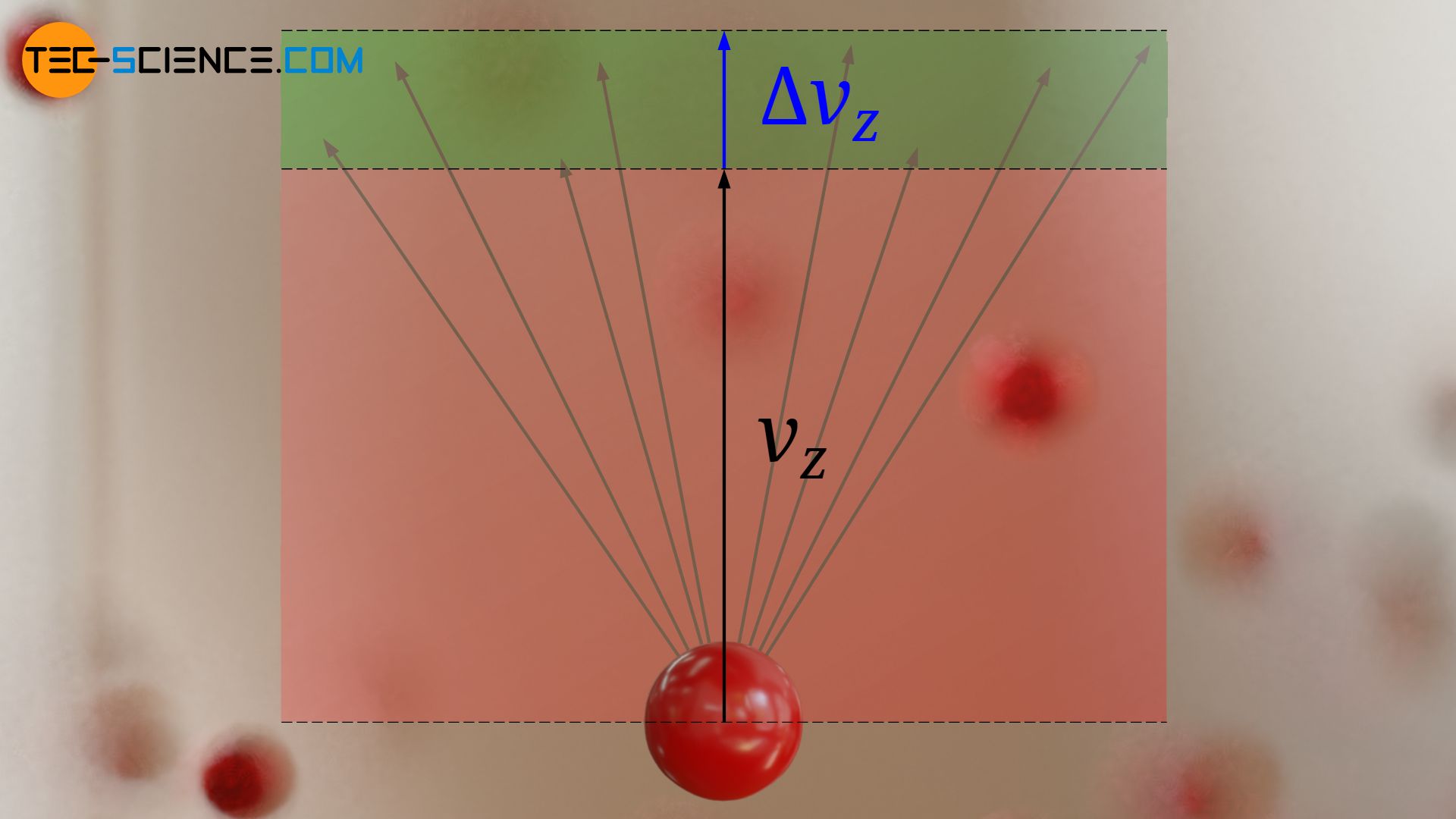
The figure below graphically shows which velocity vectors are to be considered if a speed v_z and an interval Δz are given. All vectors whose arrowheads lie within the green marked area and thus with their z-components between v_z and v_z+Δz would be considered for the calculation of the frequency.

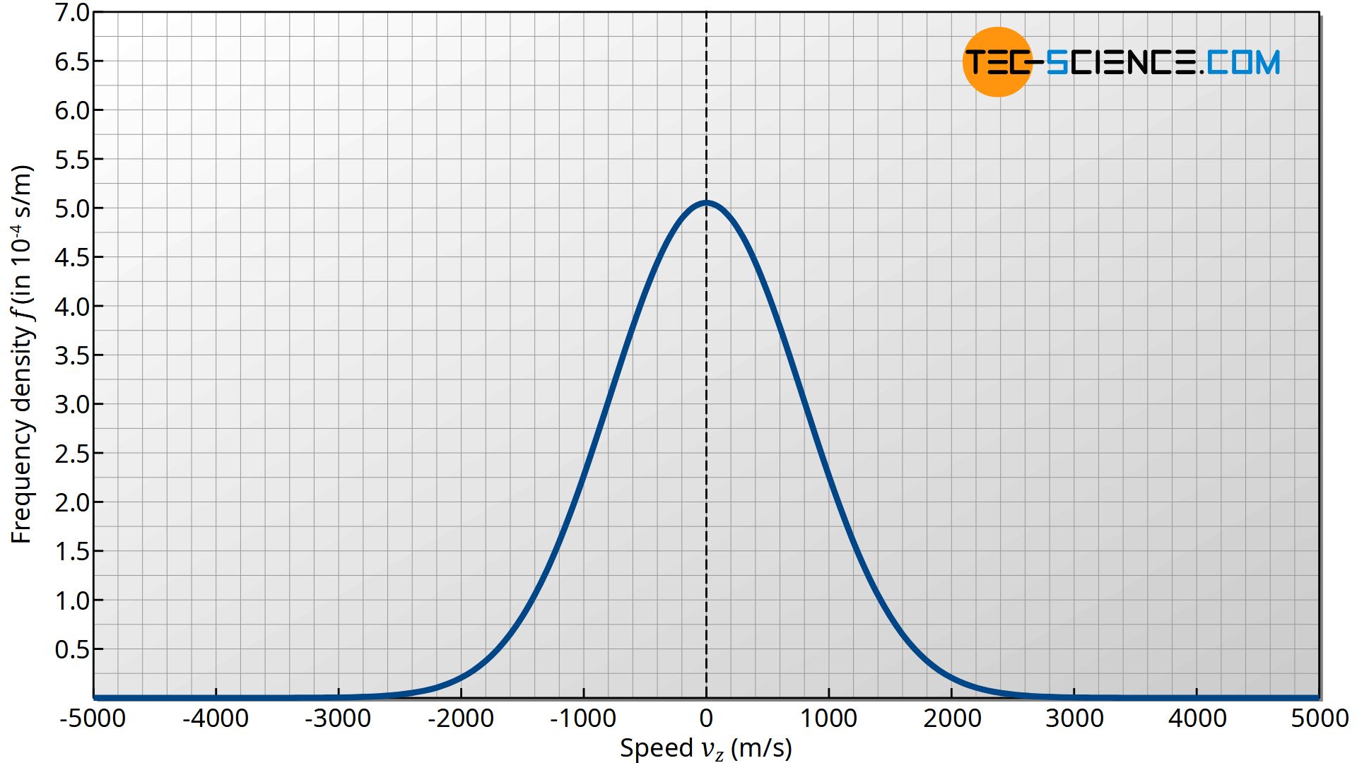
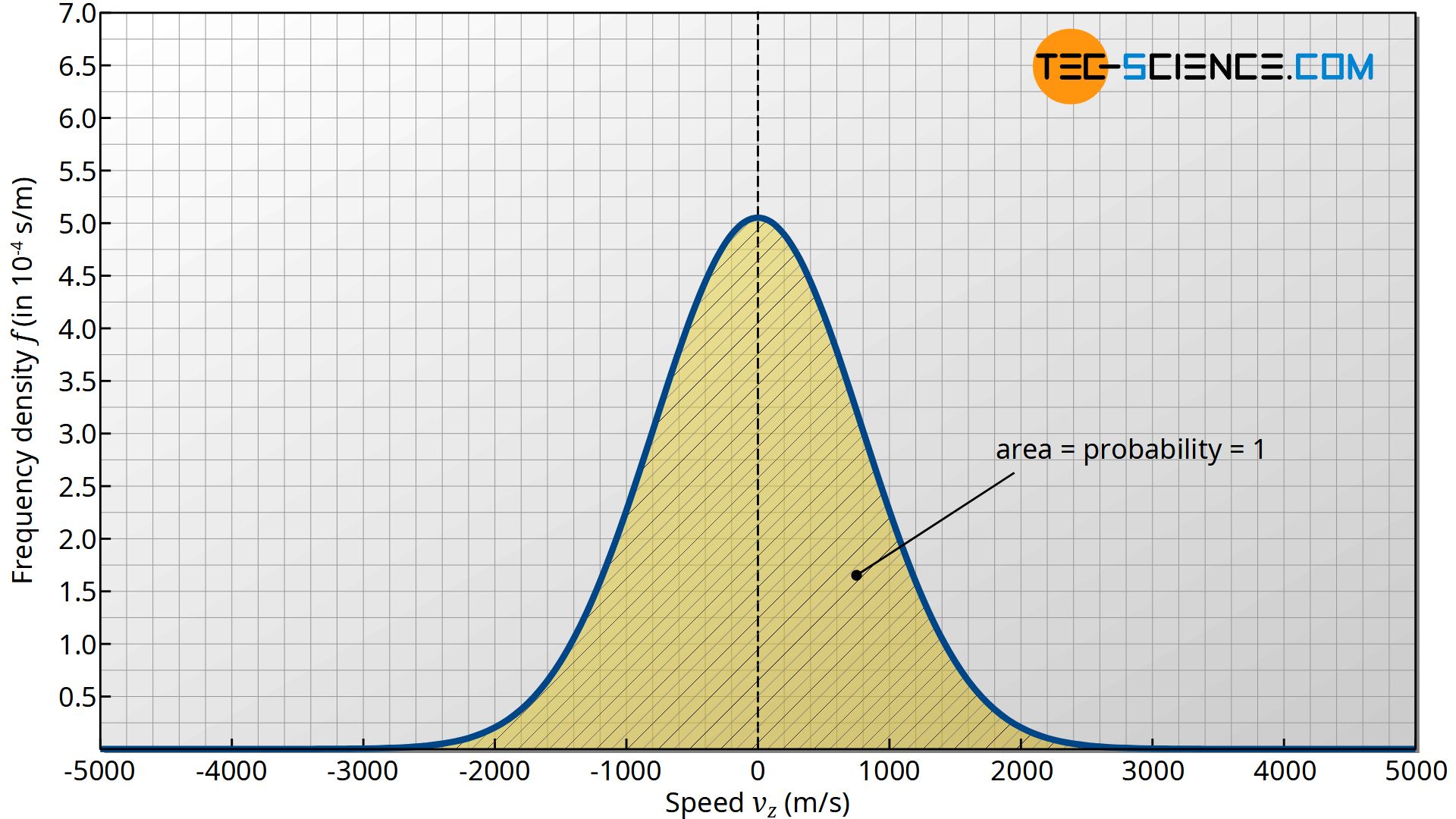
The figure below shows the qualitative course of the term f₀⋅exp(-mv_z²/2k_BT). This expression corresponds in the figurative sense to the particle density or ball density in the model conception. This function represents in this case a measure for the frequency with which certain speeds v_z are present. It is therefore called frequency density function or probability density function. The term “density” means the frequency or probability of a speed related to the corresponding speed interval:

\begin{align}
\label{norm}
&\text{frequency density} f(v_z) = \frac{\text{frequency}}{\text{speed interval}} = f_0 \cdot \exp{\left(-\dfrac{mv_z^2}{2k_BT}\right)} \\[5px]
\end{align}

Normalization of the function

Now it is necessary to determine the introduced proportionality factor in the frequency density function. This is achieved by a so-called normalization of the function. This normalization will be discussed in more detail in the following.

If equation (\ref{z}) is to be a relativ frequency (= probability!) with which a certain speed range between v_z and v_z+Δv_z is present, then the sum of the probabilities over all possible speed ranges must result in 100 %. Because if you finally sum up all occurring frequencies (probabilities) in the speed range between -∞ and +∞, then you will finally catch all molecules to 100 % (probability = 1), because any molecule must have a speed after all. Note that the molecules can have not only a positive velocity component in the z-direction, but also a negative one!

The calculation of the overall frequency (if all speeds in the range between plus and minus infinite are summed up) can be represented as follows:

\begin{align}
&\text{Overall frequency} = \sum_{-\infty}^{+\infty} f_0 \cdot \exp{\left(-\dfrac{mv_z^2}{2k_BT}\right)} \cdot \Delta v_z \overset{!}{=} 1 \\[5px]
\end{align}

Mathematically, this summation corresponds to integrating when infinitesimal speed ranges dv_z are considered instead of finite speed intervals Δv_z. With the constraint that the result must equal 1, the proportionality factor f₀ can finally be determined:

\begin{align}
&\text{Overall frequency} = \int_{-\infty}^{+\infty} \underbrace{f_0 \cdot \exp{\left(-\dfrac{mv_z^2}{2k_BT}\right)}}_{\text{frequency density function}} \cdot \text{d}v_z = \underline{f_0 \cdot \sqrt{\frac{2\pi k_B T}{m}} \overset{!}{=} 1} \\[5px]
&\boxed{f_0 = \sqrt{\frac{m}{2\pi k_B T}} }
\end{align}

The determination of the integral corresponds to the area under the graph of the frequency density function. This area was finally normalized to 1. This clearly shows that the area under the curve of the density function has the dimension of a frequency or probability!

With the factor f₀, the function for calculating the frequency is now finally normalized, i.e. fixed to the value 1, when integrating over all speeds! Thus, the frequency or probability of a speed in the range between v_z and v_z+dv_z can be calculated as follows:

\begin{align}
\label{dic}
&\boxed{\text{Frequency} = \underbrace{\sqrt{\frac{m}{2\pi k_B T}} \cdot \exp{\left(-\dfrac{mv_z^2}{2k_BT}\right)}}_{\text{frequency density} f(v_z)} \cdot \underbrace{~~~\text{d}v_z~~~}_{\text{speed interval}}} \\[5px]
\end{align}

Note that instead of macroscopic speed ranges Δv_z, infinitesimal speed intervals dv_z are now considered.

According to equation (\ref{norm}), the following function f finally applies to the frequency density or probability density:

\begin{align}
\label{f}
&\boxed{f(v_z) =\sqrt{\frac{m}{2\pi k_B T}} \cdot \exp{\left(-\dfrac{mv_z^2}{2k_BT}\right)} } ~~~\text{Frequency density function}
\end{align}

To calculate a concrete frequency F with which a speed occurs in the range between v_z1 and v_z2, the frequency density function f(v_z) must be integrated within these limits:

\begin{align}
& \boxed{\text{Frequency } F=\int_{v_{z1}}^{v_{z2}} f(v_z) ~~ \text{d} v_z} \\[5px]
\end{align}

The figure below shows the frequency density f(v_z) as a function of velocity v_z for different temperatures. Note that an area under the curve as the integral of the density function represents the frequency or probability with which the corresponding speed range is present!

Frequency density function in three dimensions

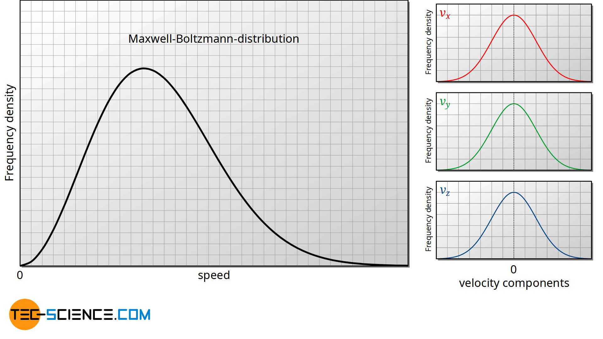
So far, the speed distribution is limited only to the velocity component of the particles in z-direction. Much more interesting however, is the distribution of the overall speeds of the molecules. For this, the frequency density function (\ref{f}) must be extended to three dimensions.

In the following, an ideal gas is considered that behaves equally in all three spatial directions. This means that the gas molecules have no direction in which they prefer to move. In particular the influence of gravity is neglected! Such a gas, that behaves the same in all directions, is also called an isotropic gas.

The velocity vector

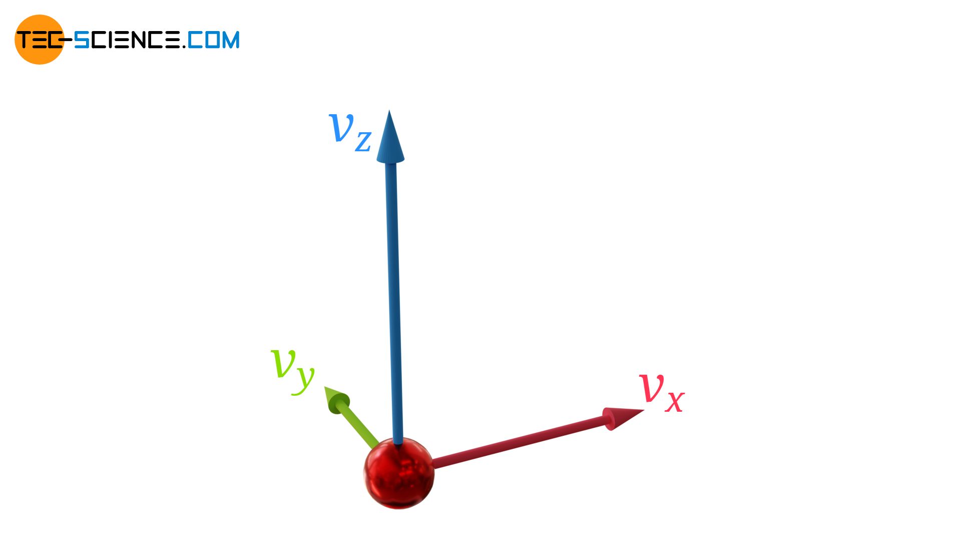
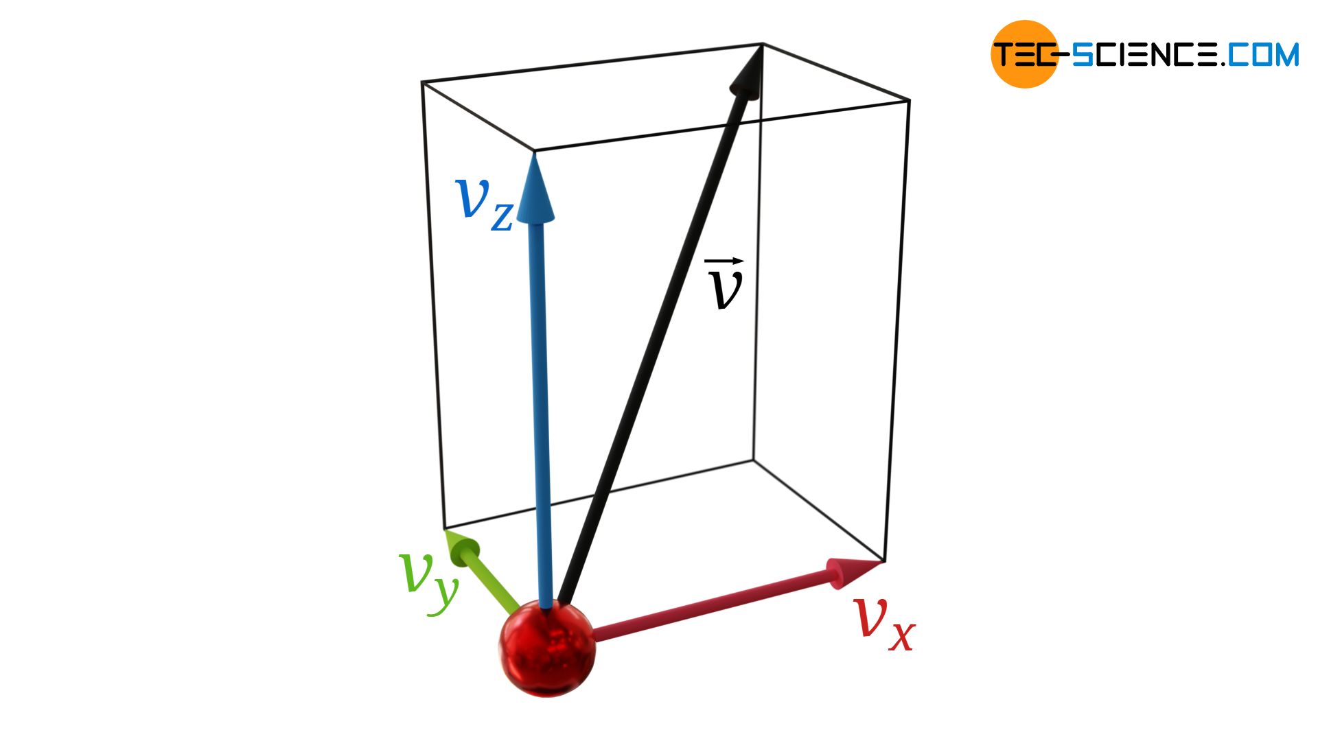
Generally, gas molecules have velocity components in all three directions (v_x, v_y and v_z). The velocity vector v of a gas particle can be represented by these three components:

\begin{align}
\vec{v} &= \begin{pmatrix}
v_{x} \\
v_{y} \\
v_{z}
\end{pmatrix}
\end{align}

For the magnitude of the velocity vector |v| or for the square |v|² applies:

\begin{align}
&|\vec{v}| = \sqrt{v_x^2+v_y^2+v_z^2} \\[5px]
\label{v22}
&|\vec{v}|^2 = v_x^2+v_y^2+v_z^2\\[5px]
\end{align}

Note that when squaring the magnitude of an vector (as done in equation (\ref{v22})), the bars that indicate the magnitude can be omitted. This leads to the same result:

\begin{align}
&\vec{v}^2 = \begin{pmatrix}
v_{x} \\
v_{y} \\
v_{z}
\end{pmatrix}
\begin{pmatrix}
v_{x} \\
v_{y} \\
v_{z}
\end{pmatrix} = v_x^2+v_y^2+v_z^2 = |\vec{v}|^2 \\[5px]
\label{v2}
&\boxed{\vec{v}^2 = v_x^2+v_y^2+v_z^2}
\end{align}

The square of a vector is therefore a scalar. We can conclude from this that by squaring a vector the information about the direction is lost. This fact will become important later!

Frequency of occurrence of a certain velocity vector

Equation (\ref{dic}) describes the frequency with which a velocity component in z-direction is present within an interval v_z and v_z+dv_z. Since an isotropic gas is assumed, this frequency distribution applies equally to each velocity component i=x,y,z:

\begin{align}
\label{dicc}
&\text{Frequency}(v_i) = \sqrt{\frac{m}{2\pi k_B T}} \cdot \exp{\left(-\dfrac{mv_i^2}{2k_BT}\right)} \cdot \text{d}v_i ~~~~~\text{for } i=x,y,z\\[5px]
\end{align}

For the velocity distribution, the question arises how often a certain vector v with given components v_x, v_y and v_z occurs within given speed intervals dv_x, dv_y and dv_z.

A simple example shows the basic procedure. In this context, it makes more sense to interpret the frequency of the occurrence of a velocity as the probability of the occurrence. We now assume that among all particles the x-component of a given velocity range occurs with a probability of 10 % (0.1) and the y-component with a probability of 5 % (0.05) and the z-component with a probability of 20 % (0.2). The overall probability that a particle has all three given velocity ranges at the same time results then from the product of the individual probabilities. In this case, the total probability is 0.1 % (0.001 = 0.1 × 0.05 × 0.2).

For the overall probability or the frequency of a certain velocity vector v (within the intervals dv_x, dv_y and dv_z equation (\ref{dicc}) must be multiplied for all three velocity components i=x,y,z:

\begin{align}
&\text{Frequency}(\vec{v}) =\text{Frequency}(v_x) \cdot \text{Frequency}(v_y) \cdot \text{Frequency}(v_z) \\[5px]
&\text{Frequency}(\vec{v}) = \left(\sqrt{\frac{m}{2\pi k_B T}}\right)^3 \cdot \exp{\left(-\dfrac{m(v_x^2+v_y^2+v_z^2)}{2k_BT}\right)} \cdot \text{d}v_x \cdot \text{d}v_x \cdot \text{d}v_x \\[5px]
\end{align}

Note that when multiplying exponential functions, the individual exponents can be summated. Therefore, the exponent now contains the sum of the squared velocity components! According to the equation (\ref{v2}), this corresponds to the square of the velocity vector:

\begin{align}
&\text{Frequency}(\vec{v}) = \left(\sqrt{\frac{m}{2\pi k_B T}}\right)^3 \cdot \exp{\left(-\dfrac{m\vec{v}^2}{2k_BT}\right)} \cdot \text{d}v_x \cdot \text{d}v_x \cdot \text{d}v_x \\[5px]
\end{align}

Frequency of occurrence of a certain speed

How is the equation above to be interpreted? If one gives a velocity vector v and for each velocity component a certain range dv_i within which the individual components can vary, then the frequency (probability) with which all the possible velocity vectors are present is determined by that equation. The heads of the velocity vectors to which the frequency is related all lie within the “volume” spanned by dv_x, dv_y and dv_z (see Figure: Interpretation of the speed interval as a spherical shell).

However, the equation also shows that the information about the direction of a velocity vector is lost on the right side of the equation. Only the square of the velocity vector appears and – as already mentioned – this is a scalar! All velocity vectors that have the same magnitude thus occur with the same frequency (since all these vectors have the same scalar value v²).

This is a good thing, because in the end it is assumed that the direction of the velocity does not play a role in the frequency distribution! Finally, an isotropic gas was assumed, in which the probabilities for the occurrence of certain velocities should not depend on the direction! For the frequency distribution the direction of the velocity is not decisive but only the speed!

The arrow symbol that usually denotes a vector can therefore be omitted in the equation above, so that v only refers to the magnitude of the velocity (molecular speed of a molecule):

\begin{align}
\label{g}
&\text{Frequencty }v = \underbrace{\left(\sqrt{\frac{m}{2\pi k_B T}}\right)^3 \cdot \exp{\left(-\dfrac{mv^2}{2k_BT}\right)}}_{\text{frequency density}} \cdot \underbrace{\text{d}v_x \cdot \text{d}v_x \cdot \text{d}v_x}_{\text{three-dimensional speed interval}} \\[5px]
\end{align}

Instead of specifying certain intervals of dv_x, dv_y and dv_z for each velocity component, it would make sense to specify a single interval dv for the speed. For this purpose a relationship between these individual intervals must be found.

Therefore equation (\ref{g}) is interpreted graphically. If a speed v is given and intervals dv_x, dv_y and dv_z are allowed, within which the components of all possible velocity vectors can vary, then a three-dimensional spherical shell results. The thickness of this spherical shell corresponds to the interval dv within which the given speed v can vary.

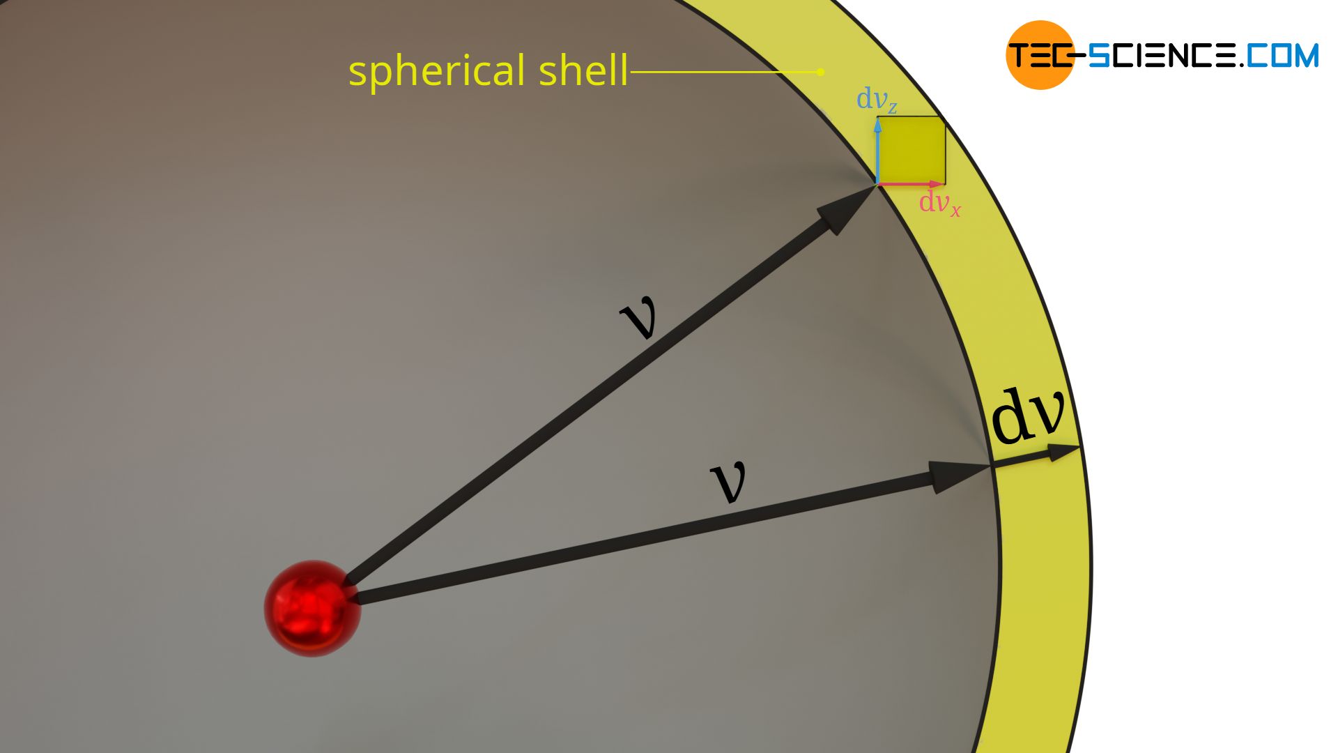
Thus, the three-dimensional speed interval in equation (\ref{g}) (defined by dv_x, dv_y and dv_z) can be replaced by a spherical shell with radius v and thickness dv. This shell is limited by two concentric spheres. Due to the infinitesimal distance between the two spheres, the volume of the sphere (volume in a velocity space!) can be determined from the product of the area of the sphere 4π⋅v² and the distance dv between the spherical shells:

\begin{align}
&\text{three-dimensional speed interval} = 4\pi v^2 \cdot \text{d}v \\[5px]
\end{align}

If this three-dimensional speed interval is used in equation (\ref{g}), then the following equation applies:

\begin{align}
&\text{Frequency} =\left(\sqrt{\frac{m}{2\pi k_B T}}\right)^3 \cdot \exp{\left(-\dfrac{mv^2}{2k_BT}\right)} \cdot \overbrace{\text{d}v_x \cdot \text{d}v_x \cdot \text{d}v_x}^{4\pi v^2 \cdot \text{d}v } \\[5px]
&\boxed{\text{Frequency} = \underbrace{\left(\sqrt{\frac{m}{2\pi k_B T}}\right)^3 \cdot 4\pi v^2 \cdot \exp{\left(-\dfrac{mv^2}{2k_BT}\right)}}_{\text{frequency density }f(v)} \cdot \underbrace{\text{d}v}_{\text{speed interval}}} \\[5px]
\end{align}

This equation finally describes the frequency or probability with which a certain speed v is present within the speed interval dv. As already explained for equation (\ref{z}), a density function f(v) can be defined at this point, which represents a measure for the frequency of an existing speed related to the speed interval dv. This distribution function is finally called Maxwell-Boltzmann distribution:

\begin{align}
\label{max}
&\boxed{f(v) = \left(\sqrt{\frac{m}{2\pi k_B T}}\right)^3 \cdot 4\pi v^2 \cdot \exp{\left(-\dfrac{mv^2}{2k_BT}\right)}}~~~~~\text{Maxwell-Boltzmann distribution} \\[5px]
\end{align}

For the calculation of a specific frequency F with which a speed occurs in the range between v₁ and v₂, the frequency density function f(v) must be integrated within these limits:

\begin{align}
& \boxed{\text{Frequency } F=\int_{v_{1}}^{v_{2}} f(v) ~~ \text{d} v} \\[5px]
\end{align}

The figure below shows the course of the Maxwell-Boltzmann distribution f(v) as a function of speed v for different temperatures. Note that the area under the curve (as the integral of the density function) represents the frequency or probability with which the corresponding speed range is present!

More detailed explanations on the statement of this distribution function can be found in the article “Maxwell-Boltzmann distribution“.

The apparent contradiction

If one compares the Maxwell-Boltzmann distribution with the distribution of the velocity components, an apparent contradiction appears at first glance. How can the frequency density of the individual components have a maximum at v=0, while in the Maxwell-Boltzmann distribution there is a minimum at v=0 (more precisely, the frequency density is zero). If there is a high probability that the velocity components are zero, shouldn’t the probability for a speed of zero also be quite high?

At this point it is important to interpret the diagrams correctly. The diagrams do not show the frequency or probability but the frequency density or probability density. For an interpretation whether a velocity component occurs rarely or frequently, the speed interval must also be considered (i.e. the area under the curve!).

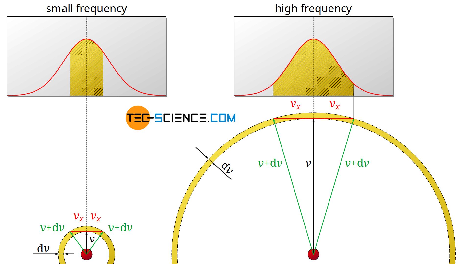
The following two-dimensional example is intended to illustrate this and resolve the apparent contradiction. A relatively low speed v (see figure on the left) and a relatively high speed v (see figure on the right) are considered. For both cases an equally large speed interval dv is given, within which the speed can vary. This interval is graphically represented by a spherical shell around the velocity vector v.

Question: In which speed range can more particles be found; in the one with the low speed (left side of the figure) or in the one with the higher speed (right side of the figure)?

According to the argumentation with the frequency distribution of the velocity components, one would probably conclude that low velocity components are more likely than large ones. Therefore, there should be more particles with lower speeds than particles with higher speeds (in this argument the frequency density is mistakenly considered as frequency).

However, if one looks at the graphic representation of the two cases, the opposite becomes apparent. In order for the given speeds v to lie within the permissible ranges dv, the x-components v_x can vary to a certain degree. Graphically, a velocity vector v+dv whose arrowhead is located on the outer spherical shell would just be permissible (shown as a green arrow). The corresponding velocity component v_x is represented by a red arrow.

As the comparison shows, at a high speed v the x-component can obviously vary within a much larger range without exceeding the speed range dv. This means that considerably more x-components are possible. The frequency distribution of the velocity components shows how often these occur in concrete terms. However, the area under the curve must be considered and not the frequency density itself (note that the area under the curve indicates the concrete frequency)! So you have to interpret the diagrams correctly and above all you must not equate the frequency density with a frequency!

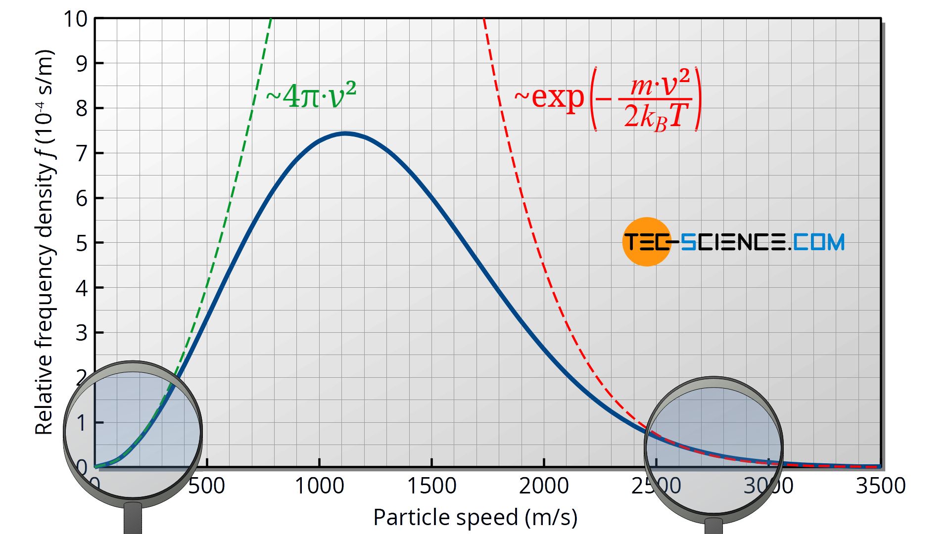
In this case, the higher speed v is therefore present much more frequently (since the permissible x-components are represented more frequently) than the lower speed. From a mathematical point of view, this is due to the quadratic influence of the speed in the Maxwell-Boltzmann distribution function (which is caused by the “spherical shell” 4π⋅v²)!

Now it also becomes clear why an extremely low speed of v≈0 is almost non-existent according to the Maxwell-Boltzmann distribution. This would mean that the velocity components would also vary only in an extremely small range. The frequency that such a small velocity range is present is extremely low (very small area under the frequency density function of the components).

At this point, the question arises why the Maxwell-Boltzmann distribution flattens out at all if, as argued above, higher speeds should be present more often than lower ones. This argumentation is of course only valid to a certain degree. As the frequency distribution of the individual components also shows, the frequency density decreases with increasing speed. This means that too high speeds are not strongly represented anyway due to the limited frequency. Mathematically, this is due to the exponential influence of the speed in the Maxwell-Boltzmann distribution function (see red dotted line in the figure above)!