Learn more about experimentally determining the velocity distribution of molecules in gases in this article.
Introduction
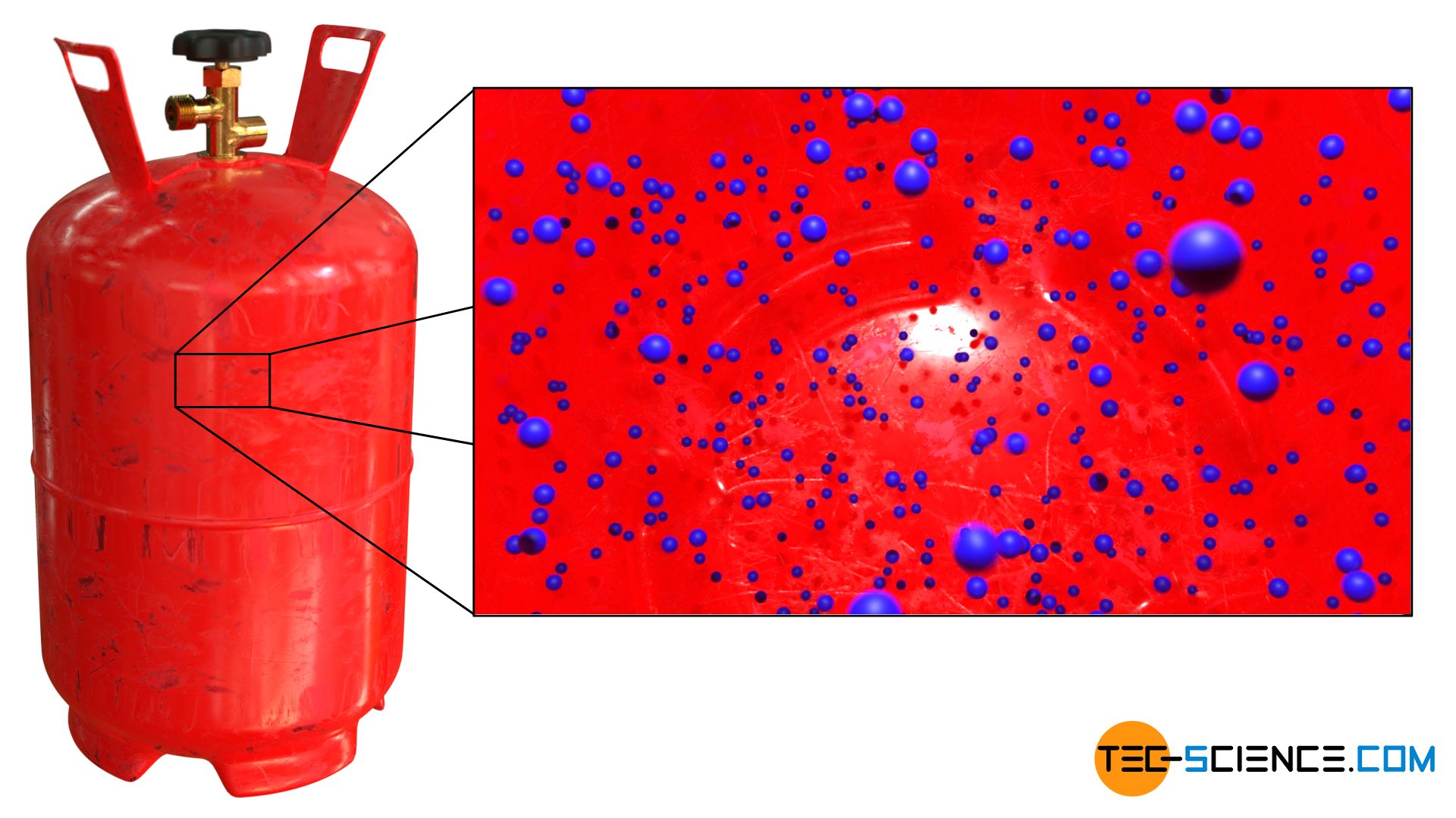
As already explained in the article Temperature and particle motion, the temperature of a gas is a measure of the kinetic energy of the particles it contains. Even at a constant temperature, however, not all the particles have the same speed. After all, in a gas at the atomic level there are permanent collisions between the particles. Some particles are slowed down and others are accelerated by the collisions. Thus, particles with different velocities can be found in a gas.
The question arises how the speeds of the particles in a gas can be determined experimentally in order to then make a statement about the velocity distribution. In the following, an experiment will be explained in more detail and its result will be discussed.
Experimental setup
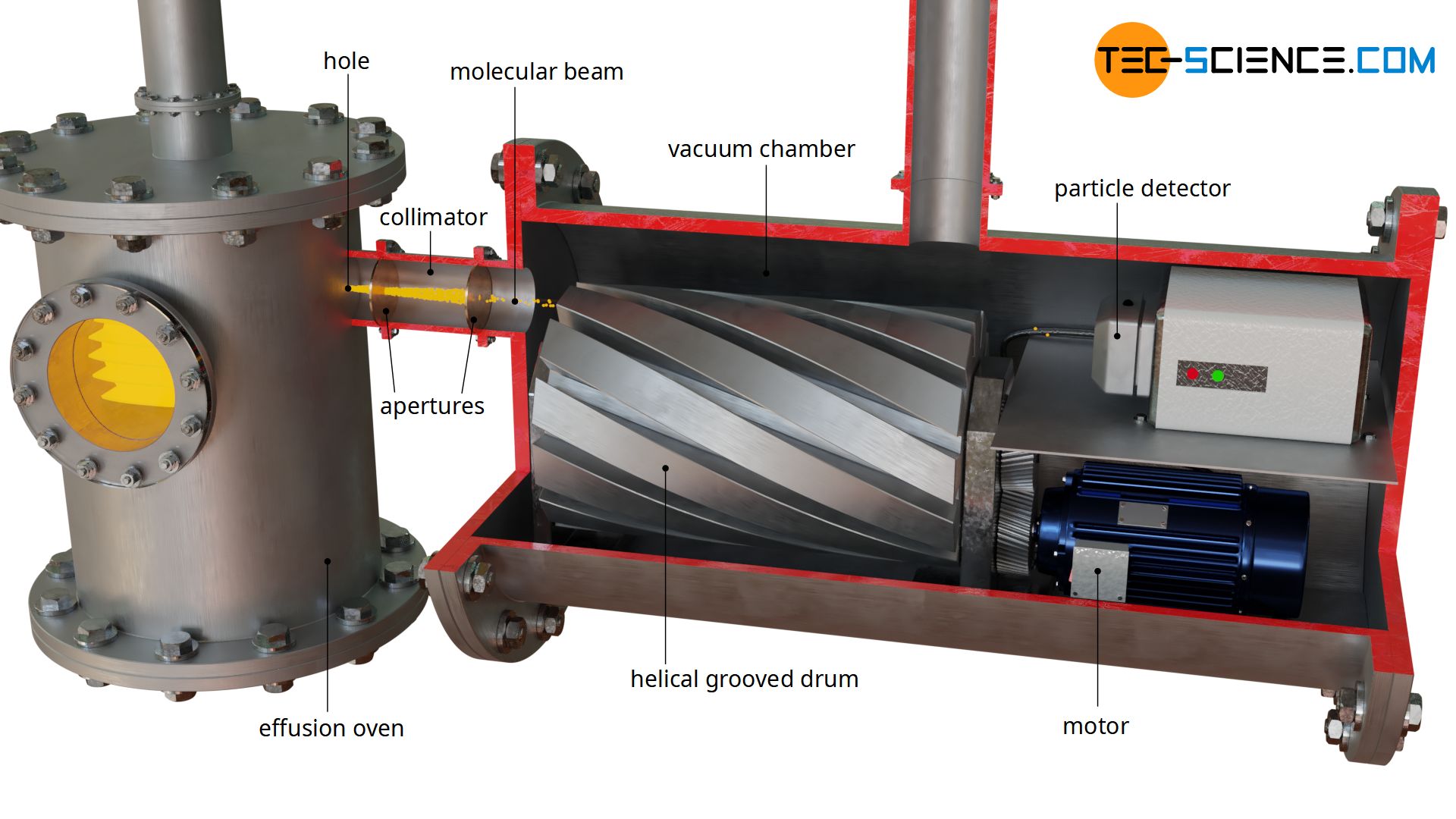
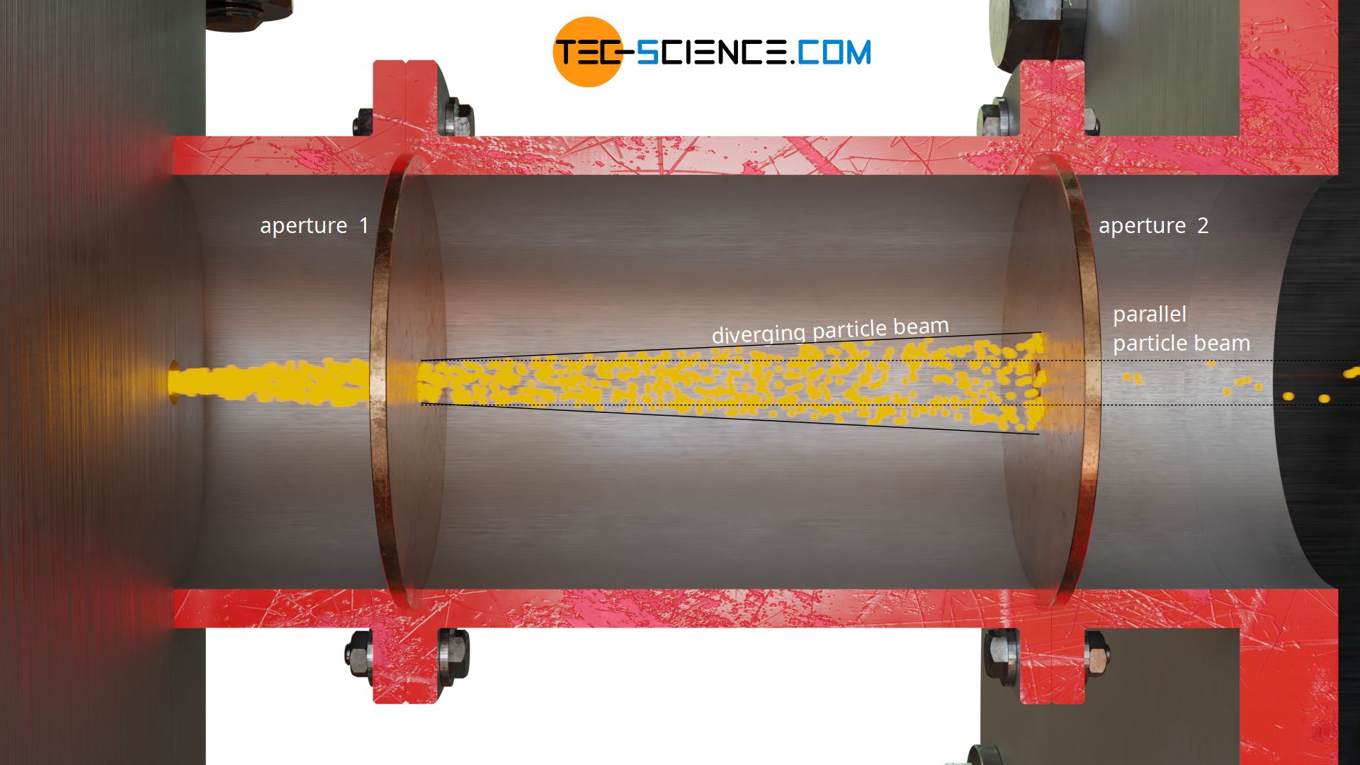
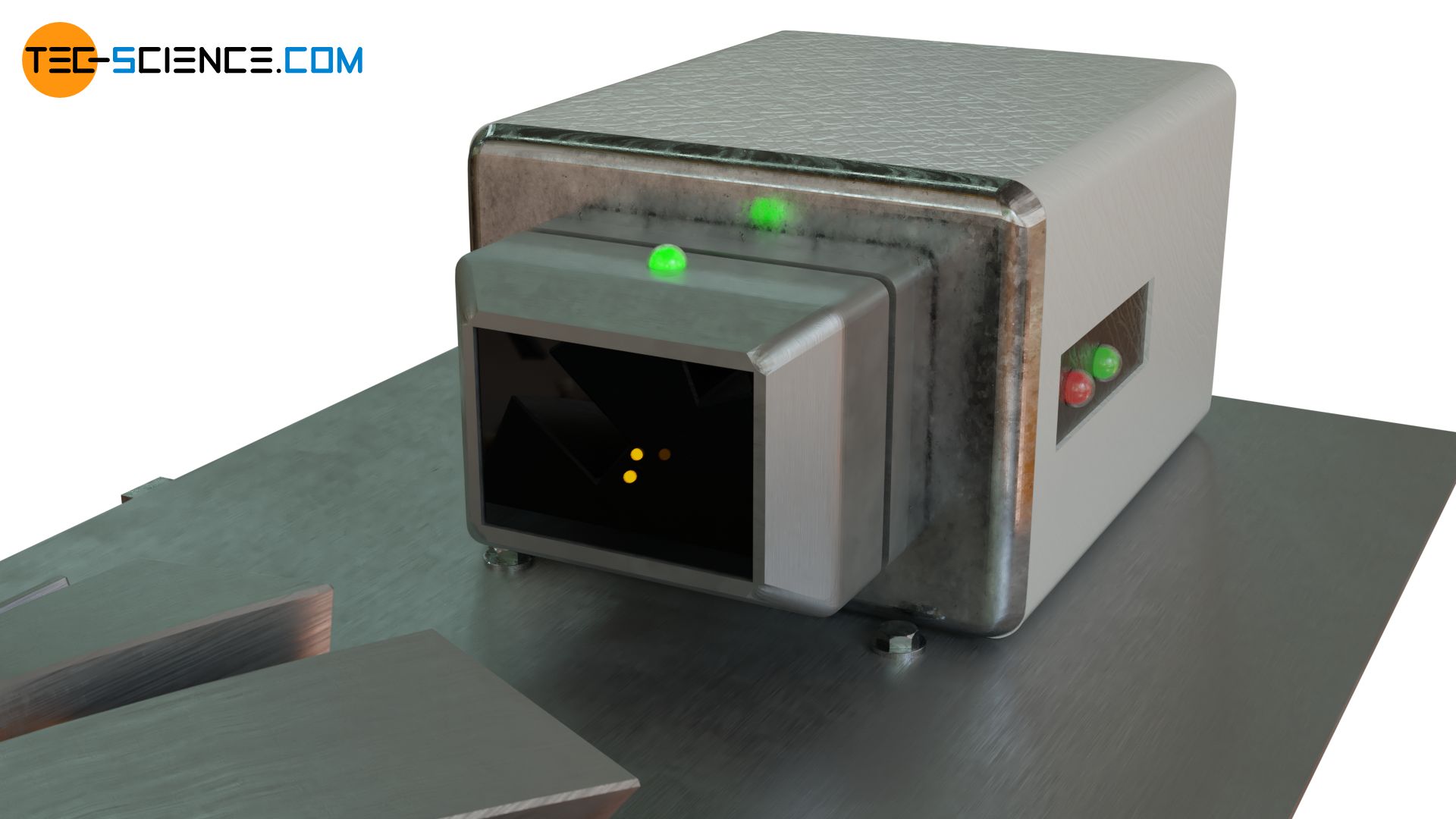
To measure the velocity of particles in a gas, a substance is first evaporated in an effusion oven and heated to a constant temperature. The gas molecules can pass through a hole in the oven in different directions. A particle beam is then generated with the use of two apertures (also called collimator). In this molecular beam, the particles move in a common direction, but at different speeds.
The speed distribution of the particles in the unidirectional stream is representative of the speed distribution of the entire gas, even if same particles were filtered out by the collimator. Ultimately, there is no direction in which the particles prefer to move in the gas. Therefore, the speed distribution in any direction is representative for the entire gas.
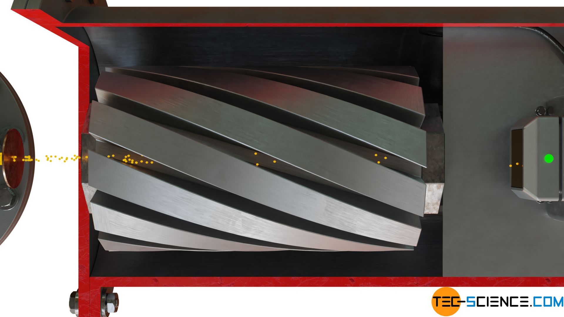
The molecular beam is now directed onto a rotating drum. At the circumference of this drum, several helical grooves are milled in axial direction (analogous to the threads of screws). Only particles whose speeds are within a certain range pass through the slotted drum at a given rotational speed. Particles that are too fast will hit the left side of the groove. If particles are too slow, they will collide with the right side of the groove.
The speed of interest can be controlled by varying the rotational speed of the drum. If the speed of the drum is high, only particles with a higher speed will pass through the apparatus. At low rotational speed, however, only particles with low speed will pass through. This experimental setup of the slotted discs thus serves as a velocity selector (speed filter). So that the gas particles to be measured are not influenced in their velocity by collisions with air molecules, the entire apparatus must be in a vacuum.
In order to obtain the distribution of the different speeds, the respective number of particles passing through the speed filter must be determined at different speeds. This is achieved with a particle detector that measures the frequency of impact.
Note: Due to the finite size of the groove width, the speed of the particles passing through the experimental setup may vary within certain limits. Therefore, it is not possible to measure the exact speeds of the gas particles, but only to analyze speed ranges. However, this is quite sufficient for the representation of a speed distribution, as will be shown later.
Due to the measuring method only velocity ranges can be assigned to a concrete number of particles!
Experimental Results
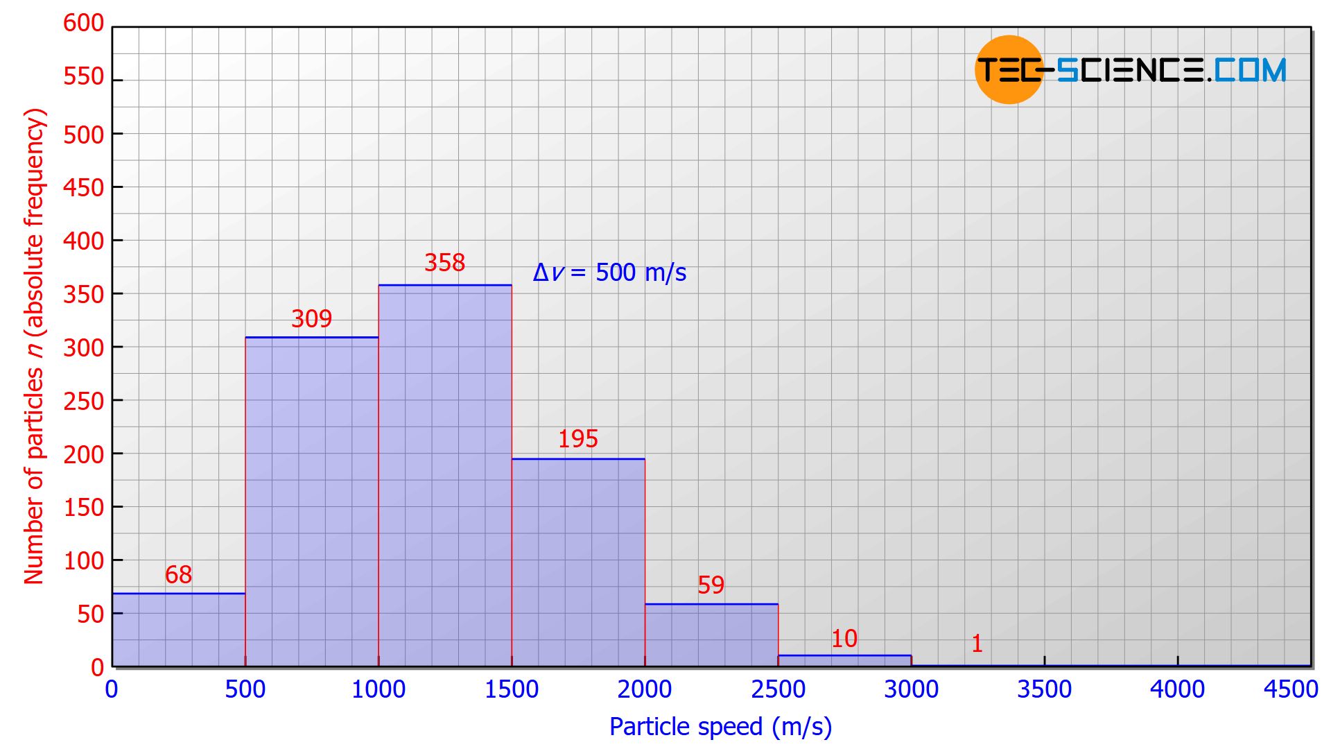
A gas usually contains innumerable particles. To better illustrate the speed distribution, we will therefore assume a number of 1000 gas particles in the following. Helium is assumed to be the gas, at a temperature of 273 K (0 °C). The speed intervals to be investigated are 500 m/s each. In this case, the following statistical distribution would typically result:
- 68 particles would have a speed in the range between 0 m/s and 500 m/s,
- 309 particles would be in the speed range between 500 m/s and 1000 m/s,
- 358 particles would be measured in the interval between 1000 m/s and 1500 m/s,
- 195 particles would have a speed in the interval between 1500 m/s and 2000 m/s,
- 59 particles would be in the speed range between 2000 m/s and 2500 m/s,
- 10 particles would have a speed in the range between 2500 m/s and 3000 m/s,
- 1 particle would show a speed greater than 3000 m/s.
Experimental evaluation
Histogram of the speed distribution
This measurement results can be evaluated in a diagram that lists the speed on the horizontal axis and the number of particles on the vertical axis. In such a diagram, the height of a bar represents the number of particles whose speeds lie within the corresponding width of the bar.
Such a graphical representation of a frequency distribution within so-called bins* is also called a histogram.
*) in the present case, the different speed intervals serve as the bins.
The histogram gives a very clear insight into the velocity distribution, but there is no generalization to any velocity intervals. With this diagram form, for example, it is not possible to deduce the number of molecules in the speed range between 1300 m/s and 1600 m/s. Based on the histogram, another form of representation is therefore used. This will be discussed in more detail in the next section.
Dependence of the histogram on the interval width
For a meaningful and more general representation of the speed distribution, it must be noted that it is in principle impossible to directly assign a specific number of particles to a certain speed. This is because the observed velocity of a particle will never correspond to the given value up to the last decimal place. After all, you would not find a single particle that exactly has this given velocity. Even on the basis of the experimental setup, it is not possible to draw conclusions about the exact speed of the gas particles anyway, but only about speed ranges (due to the finite size of the slots).
For a higher resolution of the speed distribution, the slots in the disks could be reduced in size. This would also reduce the speed range to be filtered. This then gives a more detailed picture of how many molecules are moving in a certain speed range. The figure below shows the histogram at a velocity interval of Δv = 250 m/s and Δv = 125 m/s.
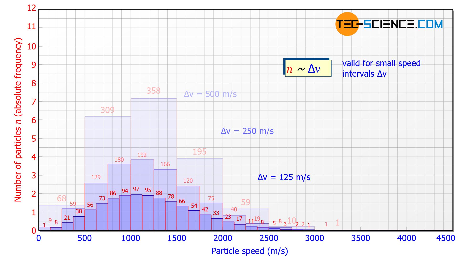
The smaller the speed interval Δv is chosen, the “flatter” the diagram will be, since the particles are divided into smaller speed ranges. For small speed intervals there is a proportional correlation between the speed interval Δv and the number of particles n in it:
\begin{align}
&n \sim \Delta v ~~~~~~~~~\text{(only valid for small speed intervals)} \\[5px]
\end{align}
The height of the bars in the histogram thus decreases by half each time the speed interval is halved. This also becomes clear, because if the interval is halved, only half of the particles in the original interval will have a higher speed and the other half a lower speed.
For small speed intervals, the number of particles within a certain speed interval (“height of the bar”) is proportional to the chosen speed interval (“width of the bar”)!
Absolute frequency distribution
For a more general representation of the speed distribution one can now use exactly this fact that speed interval and the number of particles in it are proportional to each other. This is because the quotient of the number of particles and the speed interval is then constant and no longer dependent on the chosen speed interval itself:
\begin{align}
&\frac{n}{\Delta v } = \text{constant} ~~~~\text{(frequency density)} \\[5px]
\end{align}
This quantity is also called (absolute) frequency density (unit: s/m). The animation below shows the respective histograms for different speed intervals. It becomes clear that for smaller intervals the diagram becomes smoother and smoother. For infinitely small interval widths, the result is a continuous curve that is independent of the speed intervall itself.
So it is not necessary to measure the exact velocities of the individual gas particles, a small enough speed interval is sufficient to determine the speed distribution!
In such a diagram the height of the bar no longer corresponds to the number of particles but to the area under the curve! In the figure below, the area marked in red correspond to a number of 185 particles with a speed between 1300 m/s and 1600 m/s. The area below the entire curve in the speed range between 0 and ∞ would finally correspond to 1000 particles, since all the particles would be recorded.
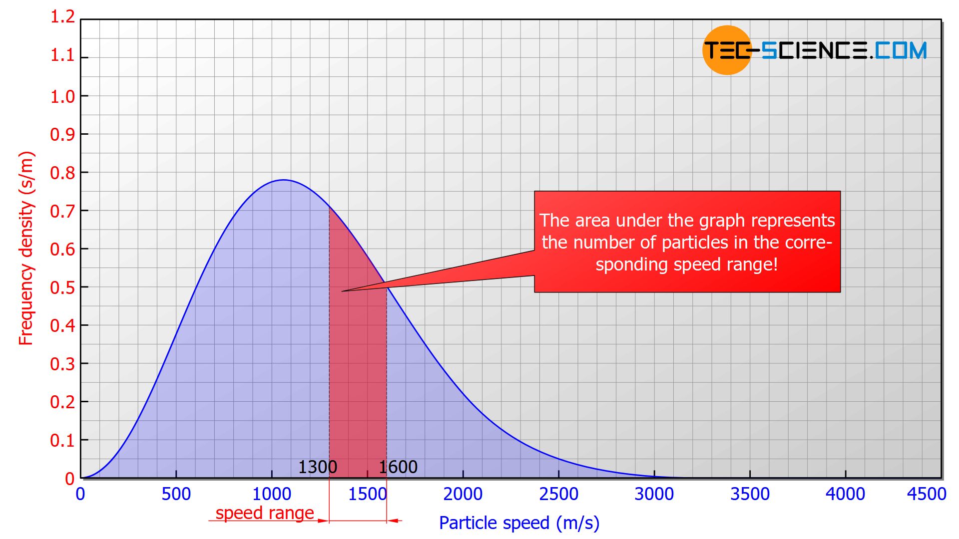
The area under the frequency distribution corresponds to the number of particles in the respective speed range!
Note that the term density in connection with the frequency density is not related to a volume or an area but to the speed! A frequency density of 5 s/m, for example, means that per 1 m/s speed interval 5 particles are found. It has to be considered that the frequency density changes with the speed. Therefore this statement is only valid for speeds close to this point.
Relative frequency distribution
The representation of the frequency distribution in the figure above is valid in this form only for a total of 1000 particles. However, the qualitative distribution would also be the same for 1 million particles. The diagram would only be stretched in height. For a general representation of the speed distribution it is therefore not practicable to plot the absolute number of particles.
The frequency distribution is usually given in percent to be independent from the total number of particles. In this case one no longer speaks of the absolute frequency distribution but of the relative frequency distribution. The size on the vertical axis is called relative frequency density.
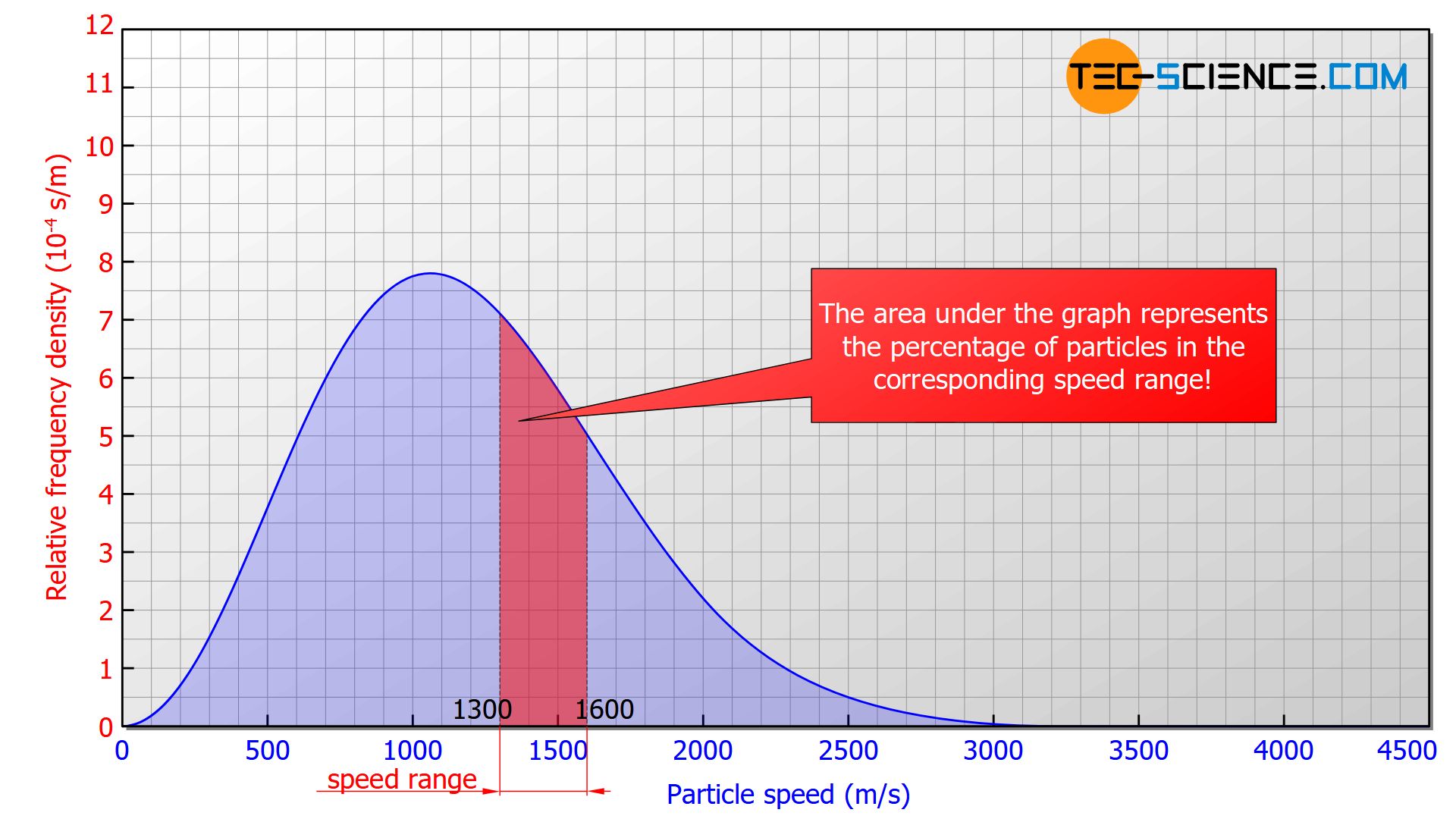
In such a diagram, the area under the graph corresponds to the percentage of molecules in the respective speed range (relative frequency). In the figure above the red marked area would correspond to 18,5 % of molecules with a speed between 1300 m/s and 1600 m/s. The area below the entire curve in the speed range between 0 and ∞ would ultimately correspond to 1 (≙ 100 %), since all the particles would be recorded.
The area under the graph corresponds to the percentage of particles in the respective speed range!
Influence of temperature on speed distribution
The figure below shows the influence of temperature on the speed distribution. For higher temperatures the speed distribution is stretched in length and squeezed in height. This results in a broader speed distribution for high temperatures, with correspondingly higher speed proportions.
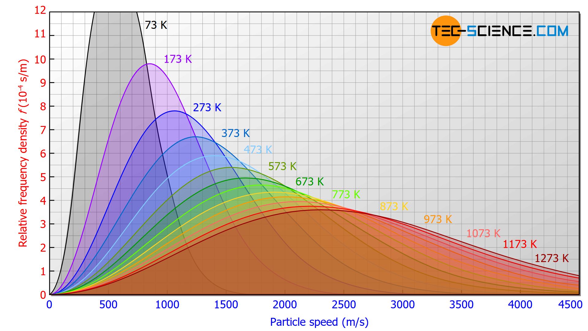
As the temperature rises, the proportion of particles with higher speeds increases!
This fact matches the statement already made in the article Temperature and particle motion that the temperature of a substance is a measure of the kinetic energy of the particles contained therein. The higher the temperature, the more energy the particles have and the faster they move. In contrast to temperature, the gas pressure has no influence on the velocity distribution (at least for an ideal gas).
The speed distribution of an ideal gas is independent of the gas pressure!
The physicists James Clerk Maxwell and Ludwig Boltzmann attempted to derive such a speed distribution on the basis of the kinetic theory of gases using statistical methods. In 1860, the two physicists finally succeeded. Therefore, such a speed distribution as shown above is also called Maxwell-Boltzmann speed distribution. The article Maxwell-Boltzmann distribution deals with this in more detail.


")
")

