With the Transient-Hot-Wire method (THW), the thermal conductivity is determined by the change in temperature over time at a certain distance from a heating wire.
Design
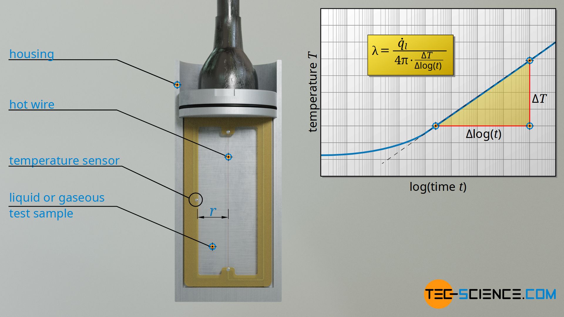
With the transient-hot-wire method, the thermal conductivity is determined on the basis of the increase in the temperature of a substance over time when it is heated by a thin hot wire. The heating wire is located directly in the test sample. Gaseous and liquid substances can be examined particularly easily, since the heating wire can be immersed in such fluids relatively easily. The substance to be examined can also be brought to different temperatures by temperature control of the apparatus. In this way the thermal conductivity can be examined as a function of temperature.
Mathematical description of the heating process
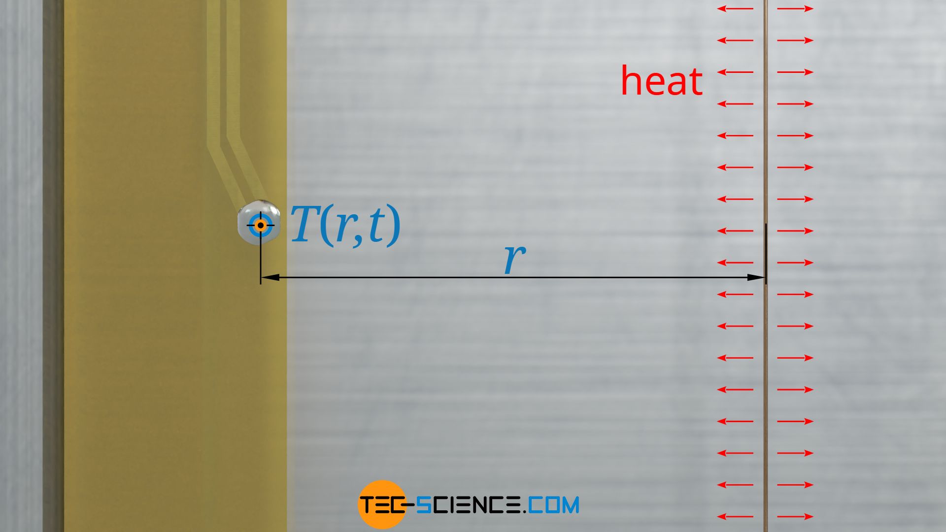
To be able to determine the thermal conductivity from the observed temperature increase, this process must first be described mathematically. From the heat equation, the following formula is obtained for a linear heat source (thin, long wire), with which the temperature T at a distance r from the heat source at a certain time t can be determined:
\begin{align}
\label{t}
& \boxed{T(r,t) = \frac{\dot q_l}{4 \pi \cdot \lambda} \cdot \left[\ln \left( \frac{4\cdot a \cdot t}{r^2}\right) -\gamma\right]} \\[5px]
\end{align}
Therein q*l denotes the specific heat output of the linear heat source (emitted heat energy per unit time and unit length). λ denotes the thermal conductivity of the surrounding medium and “a” denotes the thermal diffusivity of the substance. \gamma corresponds to Euler’s constant with a value of 0.57721. The latter expression is obtained by an approximate series expansion which is only valid if the expression r²/(4⋅a⋅t) is much smaller than 1. This is true in particular if small distances r to the hot wire are considered or/and the times t are chosen relatively large.
Testing procedure
According to the equation (\ref{d}) given below, there is a relationship between thermal conductivity and thermal diffusivity, but in equation (\ref{t}) the thermal diffusivity is in the argument of the logarithm function, so that even with this relation the upper equation cannot be solved so easily with respects to the thermal conductivity.
\begin{align}
\label{d}
& \boxed{\lambda = a \cdot \rho \cdot c_p} \\[5px]
\end{align}
Therefore, for a given distance r, one does not measure the temperature at a certain time, but the temperature difference between two points in time. In this way, neither the distance r nor the thermal diffusivity “a” plays a role:
\begin{align}
\require{cancel}
\Delta T &= T(r,t_2) – T(r,t_1) \\[5px]
\Delta T & = \frac{\dot q_l}{4 \pi \cdot \lambda} \cdot \left[\ln \left( \frac{4\cdot a \cdot t_2}{r^2}\right)-\gamma \right] – \frac{\dot q_l }{4 \pi \cdot \lambda} \cdot \left[\ln \left( \frac{4\cdot a \cdot t_1}{ r^2}\right)-\gamma\right] \\[5px]
\Delta T & =\frac{\dot q_l }{4 \pi \cdot \lambda} \cdot \left[\ln \left( \frac{4\cdot a \cdot t_2}{ r^2}\right) – \bcancel{\gamma}~ – \ln \left( \frac{4\cdot a \cdot t_1}{r^2}\right) +\bcancel{\gamma} \right] \\[5px]
\Delta T & =\frac{\dot q_l }{4 \pi \cdot \lambda} \cdot \left[\ln \left( \frac{4\cdot a \cdot t_2}{r^2}\right) – \ln \left( \frac{4\cdot a \cdot t_1}{ r^2}\right) \right] \\[5px]
\Delta T & =\frac{\dot q_l }{4 \pi \cdot \lambda} \cdot \ln \left( \frac{\frac{4\cdot a \cdot t_2}{ r^2} }{ \frac{4\cdot a \cdot t_1}{r^2} } \right) \\[5px]
\Delta T & =\frac{\dot q_l }{4 \pi \cdot \lambda} \cdot \ln \left(\frac{t_2}{t_1}\right) \\[5px]
\end{align}
\begin{align}
\label{l}
&\boxed{\lambda =\frac{\dot q_l }{4 \pi \cdot \Delta T } \cdot \ln \left(\frac{t_2}{t_1}\right)} \\[5px]
\end{align}
For the determination of the thermal conductivity λ, one only has to determine the temperature increase ΔT between two points in time t1 and t2 for a given specific heat output q*l. Note that for this formula to be valid, the distance r to the heating wire must be selected relatively small and the time measurement should not be started directly when the heating wire is switched on, but only some time later.
Evaluation of the measurement
In practice, the thermal conductivity is not only determined on the basis of two measurements, but the temperature change over time is recorded first. This curve is then displayed in a logarithmic time-temperature diagram. The thermal conductivity can then be determined from the slope of the straight line. The measuring time is usually only a few seconds, whereby temperature changes of less than 1 °C are sufficient for a reliable evaluation. Within such a short measuring time, convection currents in fluids become practically negligibleThe figure below shows a schematic representation of the temperature curve as a function of logarithmic time.
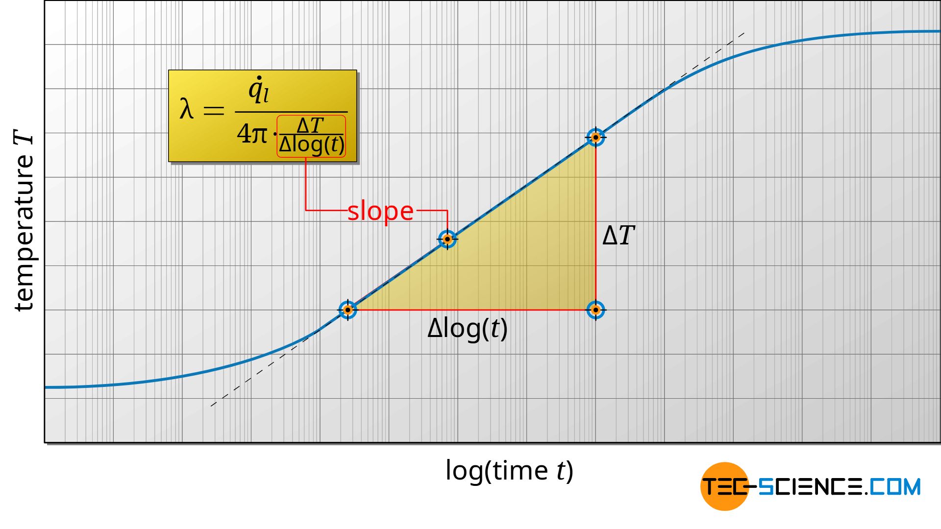
Note that the derived formulas are only valid in the linear part of the graph. This is due to the already mentioned requirement that the times must be long enough for the formulas to be valid. It must also be noted that in practice the heating wire must first heat itself before it can heat the actual test sample. For this reason, there is a non-linearity between the temperature change and the logarithmic time at the beginning of the measurement. The linearity is only present after some time. If the time is too long, however, this linearity also disappears again. This is the case when the heat has penetrated the test material, so to speak, and it then only heats up in total.
The linear dependence shown in the diagram is obtained mathematically by rearranging equation (\ref{l}):
\begin{align}
&\lambda =\frac{\dot q_l }{4 \pi \cdot \Delta T } \cdot \ln \left(\frac{t_2}{t_1}\right) \\[5px]
&\Delta T=\frac{\dot q_l }{4 \pi \cdot \lambda} \cdot \left[\ln(t_2)-\ln(t_1) \right] \\[5px]
&\Delta T=\frac{\dot q_l }{4 \pi \cdot \lambda} \cdot \Delta \ln(t) \\[5px]
\end{align}
Finally, the thermal conductivity λ is determined as follows from the slope in the linear range of the graph:
\begin{align}
&\frac{\Delta T}{ \Delta \ln(t) }=\frac{\dot q_l }{4 \pi \cdot \lambda} = \text{slope of the } T(\ln(t))\text{-diagram}\\[5px]
&\boxed{\lambda=\frac{\dot q_l}{4\pi \cdot \text{“slope”}}} \\[5px]
\end{align}
Field of application
Typically, the Transient-Hot-Wire method is used for gases and liquids whose thermal conductivities are between 0.1 and 50 W/(mK). If the thermal conductivities are too high, the diagram often does not show a linear relationship, so that no evaluation is possible.
")


")

