In this article we discuss temperature curves and heat flows through a plane wall, through a cylindrical pipe and through a hollow sphere.
Introduction
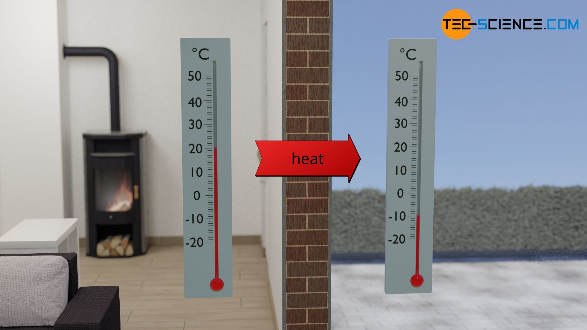
Temperature differences cause heat flows. These heat flows, in turn, cause different temperature profiles inside the considered material depending on its geometry. As an example, the following calculation will show the temperature curve for heat conduction through a plane vessel wall, through a cylindrical pipe and a hollow sphere.
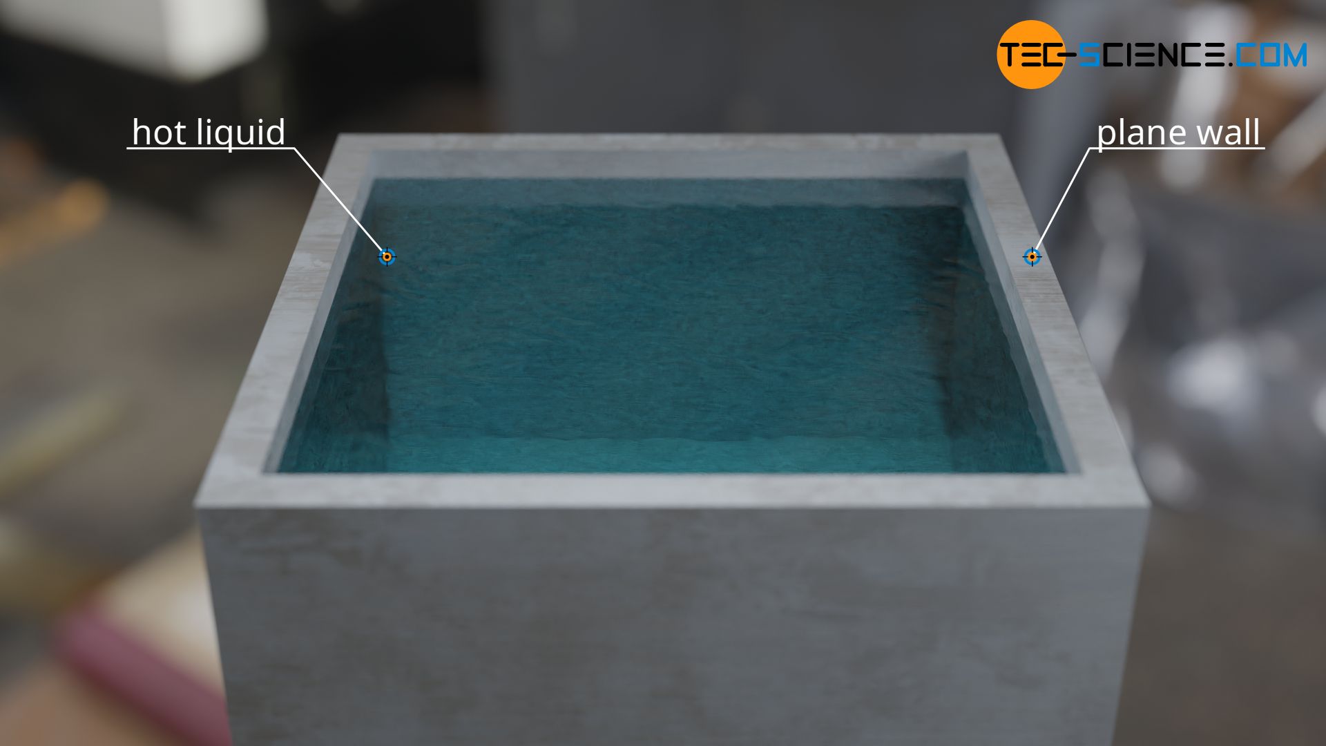
Heat flow through a flat wall is probably the most common case. An example is the heat flow through a building wall or through the vessel wall of a container of hot water.
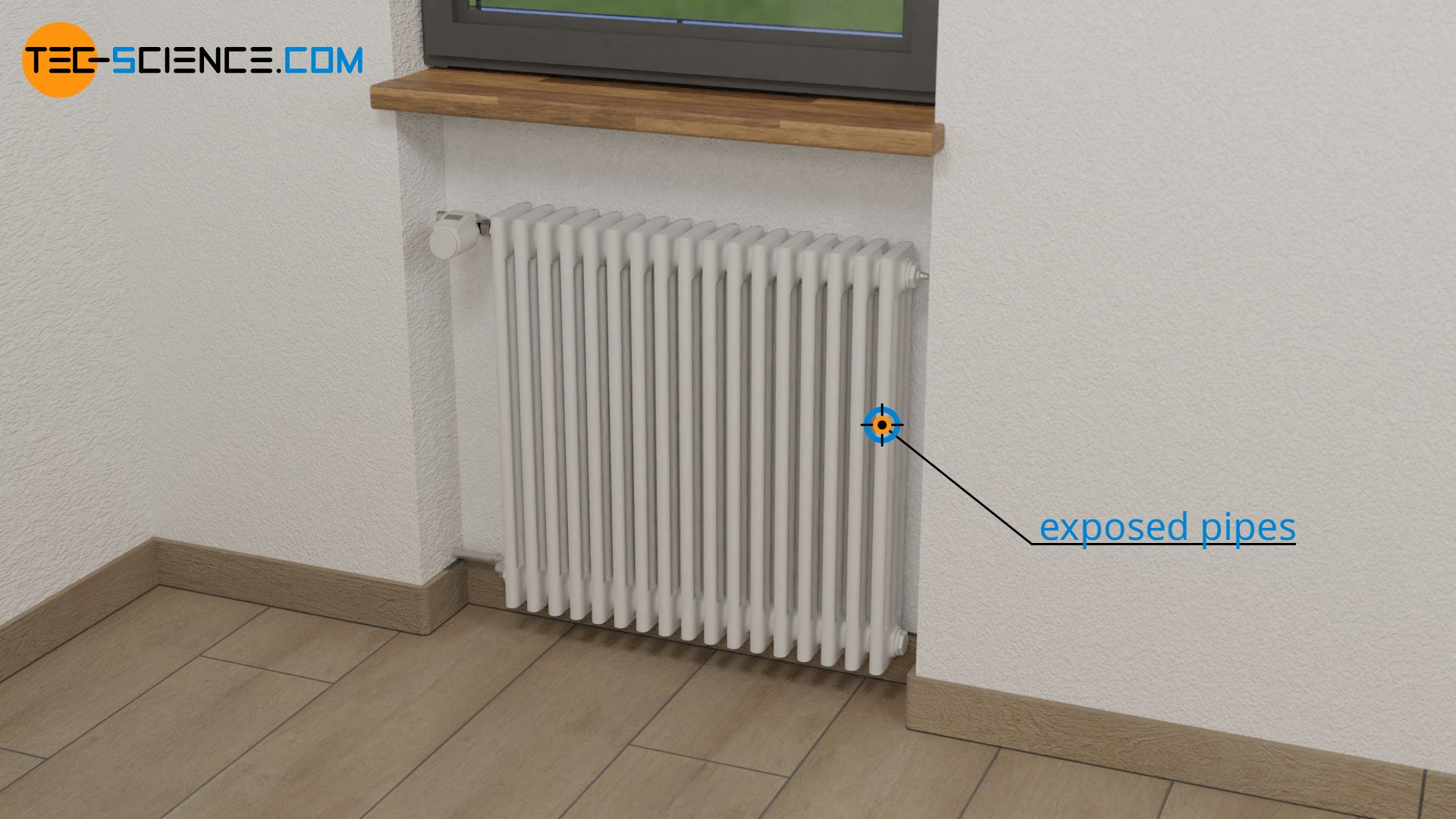
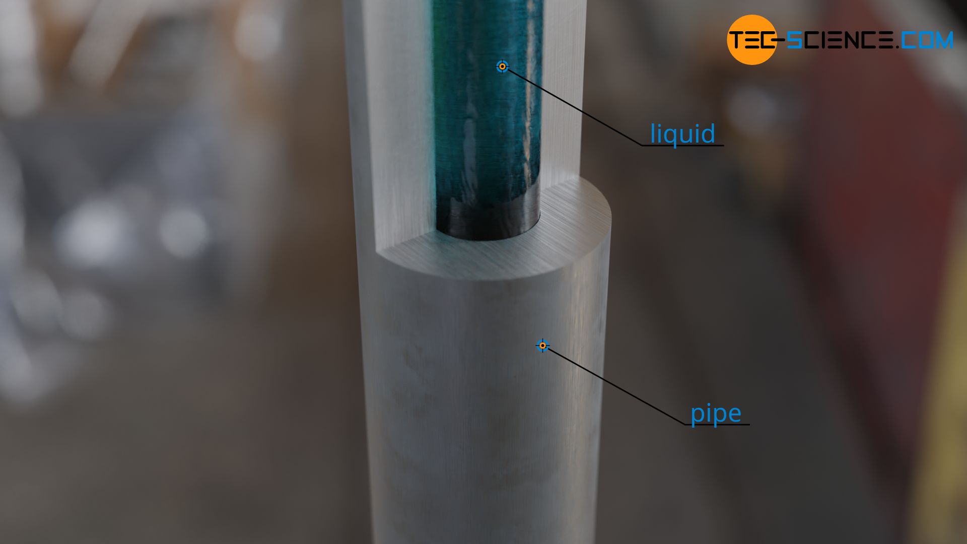
Heat flows through hollow cylinders are generally found in pipelines. The heating pipes of some radiators have such a cylindrical shape.
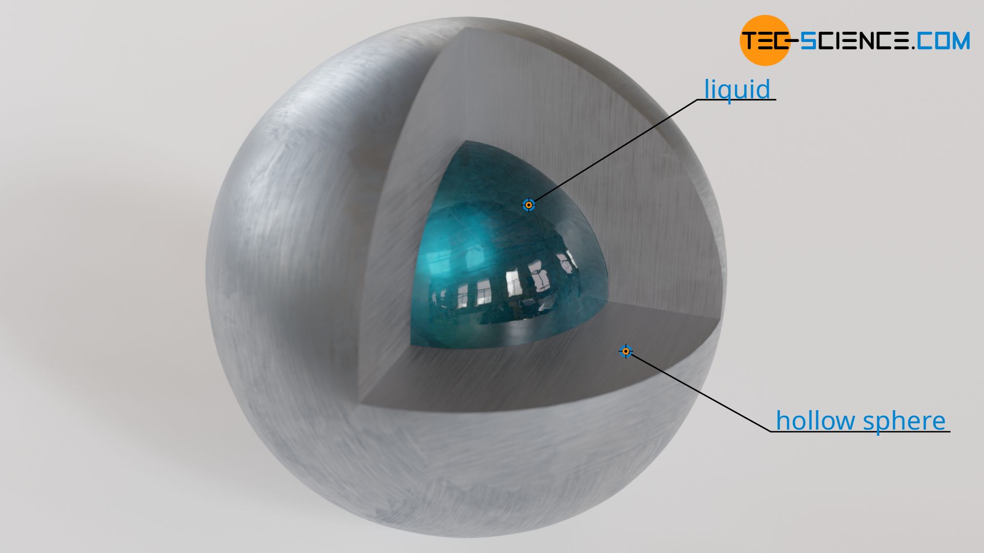
In rare cases, the geometry can also have the shape of a hollow sphere. This is the case with some special containers that store hot water in a spherical tank.
According to Fourier’s law, the rate of heat flow Q* through a surface area A depends on the temperature gradient dT/dr:
\begin{align}
&\dot Q = – \lambda \cdot A \cdot \frac{\text{d}T}{\text{d}r} \\[5px]
\end{align}
Therefore for the infinitesimal temperature change dT along a section dr applies:
\begin{align}
\label{q}
&\boxed{ \text{d}T = – \frac{\dot Q}{\lambda \cdot A} \cdot \text{d}r} \\[5px]
\end{align}
The quotient of heat flow and surface area can be regarded as heat flux q* (“heat flow density”), i.e. as heat flow per unit area:
\begin{align}
\label{qq}
&\boxed{ \text{d}T = – \frac{\dot q}{\lambda} \cdot \text{d}r} \\[5px]
\end{align}
Temperature profiles
Temperature profile inside a plane wall
For a plane wall, the surface A in the direction of the heat flow is always constant and thus not a function of the distance r. The heat flow Q* is the heat flow that is transferred to the inside of the wall and conducted through the wall. Due to the conservation of energy, this heat also passes through every imaginary intermediate plane to the same extent (in the steady state, which we assume for all examples in this article).
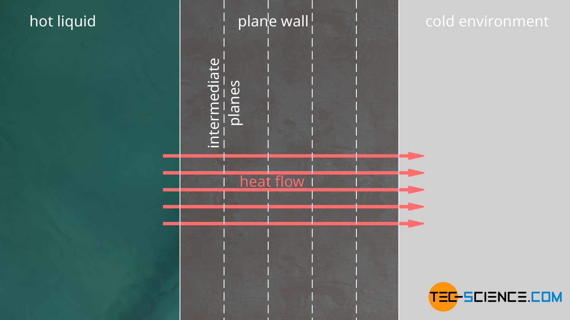
If this were not the case, the wall would either heat up by “accumulation” of heat or cool down by “removing” heat. However, we would like to consider only the case of a steady state, in which the temperature curve does not change over time. Due to the constant heat flow and the constant area through which the heat passes, we obtain a constant heat flux q*. According to the equation (\ref{qq}), this in turn means that the temperature always changes per section dr by the same amount dT. Consequently, there is a linear temperature change for a plane wall.
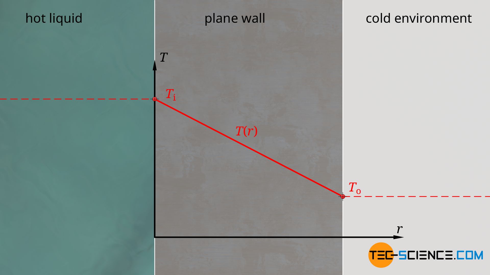
The exact course of the temperature T(r) can be determined by integrating equation (\ref{q}), whereby the thermal conductivity is assumed to be constant. Here Ti denotes the temperature on the inside of the wall at r=0:
\begin{align}
& \text{d}T = – \frac{\dot Q}{\lambda \cdot A} \cdot \text{d}r \\[5px]
& \int \limits_{T_i}^{T}\text{d}T = – \frac{\dot Q}{\lambda \cdot A} \cdot \int \limits_{0}^{r}\text{d}r \\[5px]
& [T]_{T_i}^{T}= – \frac{\dot Q}{\lambda \cdot A} \cdot [r]_{0}^{r}\\[5px]
& T-T_i= – \frac{\dot Q}{\lambda \cdot A} \cdot r \\[5px]
\label{e}
&\boxed{T(r) = T_i – \frac{\dot Q}{\lambda \cdot A} \cdot r} \\[5px]
\end{align}
The temperature changes linearly through a plane wall!
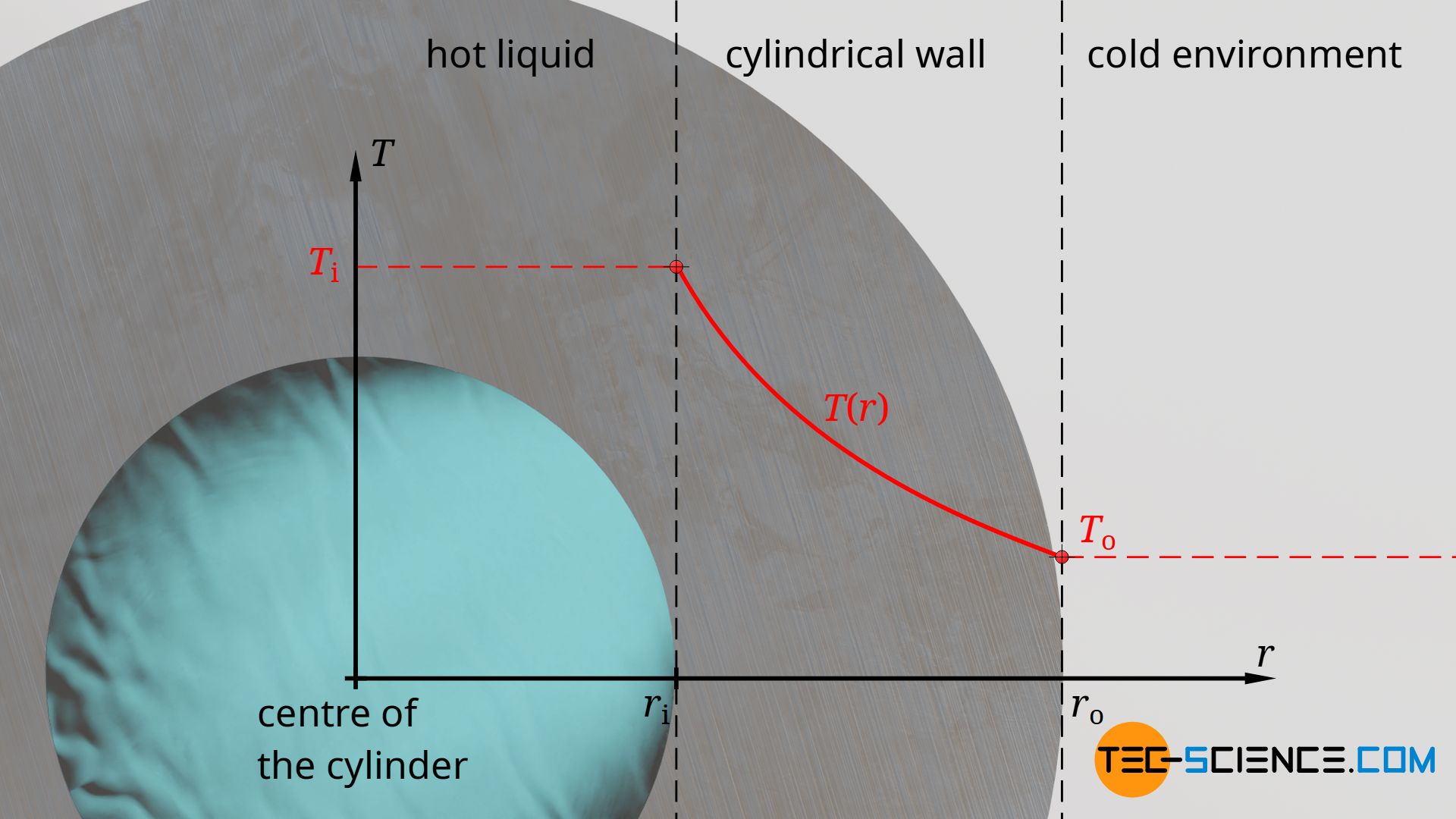
Temperature profile inside a cylindrical pipe
Even with a cylindrical wall, the heat transferred from the inside to the outside of the wall passes through every imaginary intermediate plane to the same extent (steady state!). Otherwise the pipe would heat up or cool down again. The heat flow Q* through the cylindrical wall is therefore again not a function of the coordinate r, but constant.
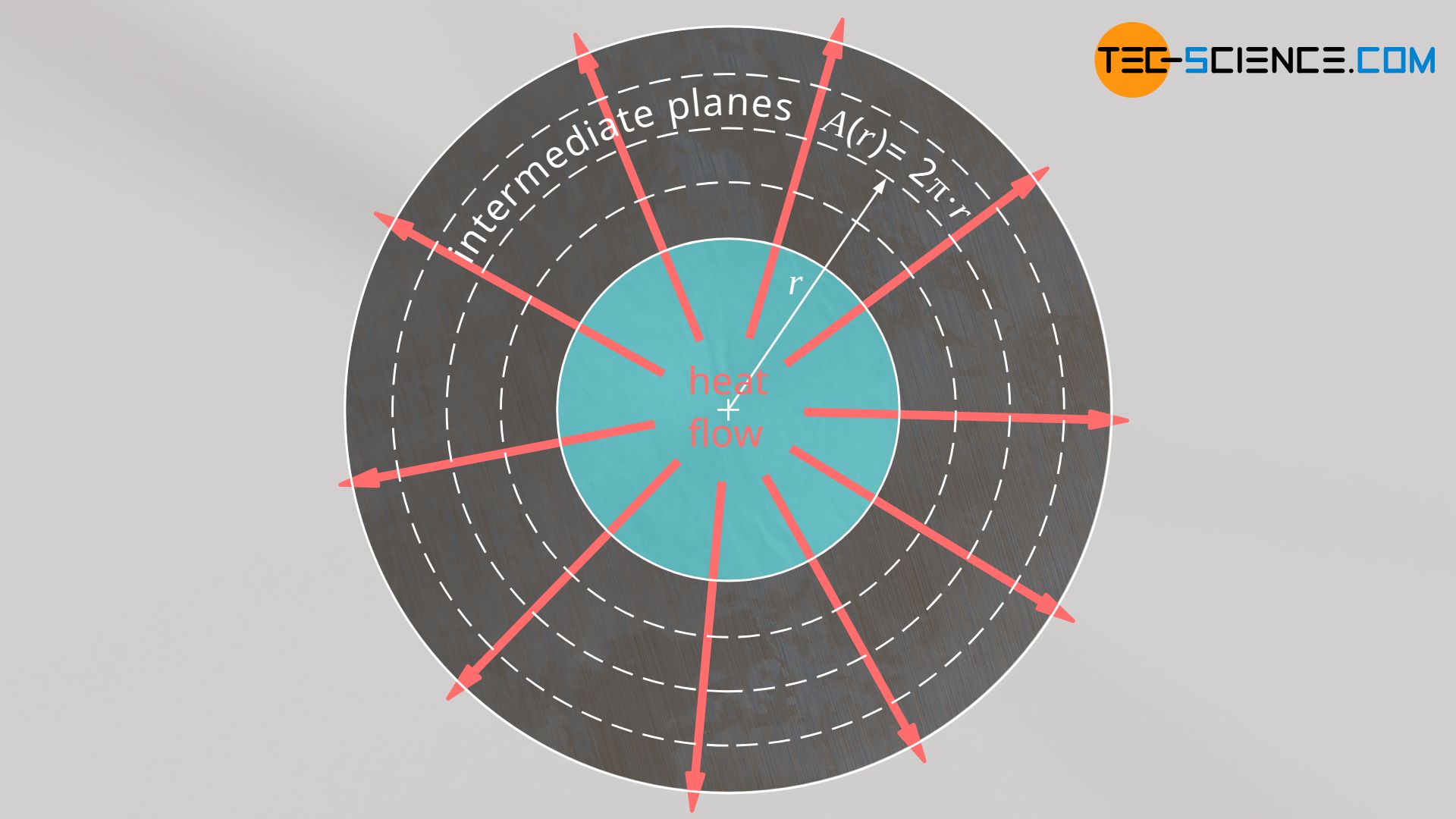
Unlike the plane wall, however, the area (of the intermediate planes) through which the heat passes changes. With larger radius r the surface area increases linearly. This in turn means that the heat flow is distributed over a larger and larger area, i.e. the heat flux decreases with increasing distance r. According to the equation (\ref{qq}) this means that the temperature changes less and less with increasing distance from the inner wall. The temperature curve therefore flattens out.
The exact course of the temperature T(r) is obtained by integrating equation (\ref{q}), whereby the thermal conductivity is again assumed to be constant. However, it must be noted that the area is now a function of the radius. Using l as the length of the cylindrical pipe, the surface area A at a distance r can be determined as follows:
\begin{align}
& A(r) = 2\pi \cdot l \cdot r \\[5px]
\end{align}
Using this function in equation (\ref{q}) and then integrating it, the following temperature curve inside the pipe is obtained:
\begin{align}
& \text{d}T = – \frac{\dot Q}{\lambda \cdot A(r)} \cdot \text{d}r \\[5px]
& \int \limits_{T_i}^{T}\text{d}T = – \frac{\dot Q}{\lambda \cdot 2\pi \cdot l } \cdot \int \limits_{r_i}^{r} \frac{\text{d}r}{r} \\[5px]
& [T]_{T_i}^{T}= – \frac{\dot Q}{ \lambda \cdot 2\pi \cdot l } \cdot \left[\ln(r)\right]_{r_i}^{r}\\[5px]
& T-T_i= – \frac{\dot Q}{\lambda \cdot 2\pi \cdot l} \cdot \left[\ln(r)-\ln(r_i)\right] \\[5px]
& T-T_i= – \frac{\dot Q}{\lambda \cdot 2\pi \cdot l} \cdot \ln\left( \frac{r}{r_i}\right) \\[5px]
\label{z}
& \boxed{T(r)= T_i – \frac{\dot Q}{\lambda \cdot 2\pi \cdot l} \cdot \ln\left( \frac{r}{r_i}\right)} \\[5px]
\end{align}
The temperature through a cylindrical wall changes logarithmically!
Temperature profile within a hollow sphere
For example, if there is a hot liquid inside a spherical vessel, heat will penetrate through the wall of the sphere to the outside. In the steady state, the heat passes through every imaginary intermediate plane to the same extent. However, the area (of the intermediate planes) through which the heat passes increases with increasing radius, so that the heat flux decreases accordingly.
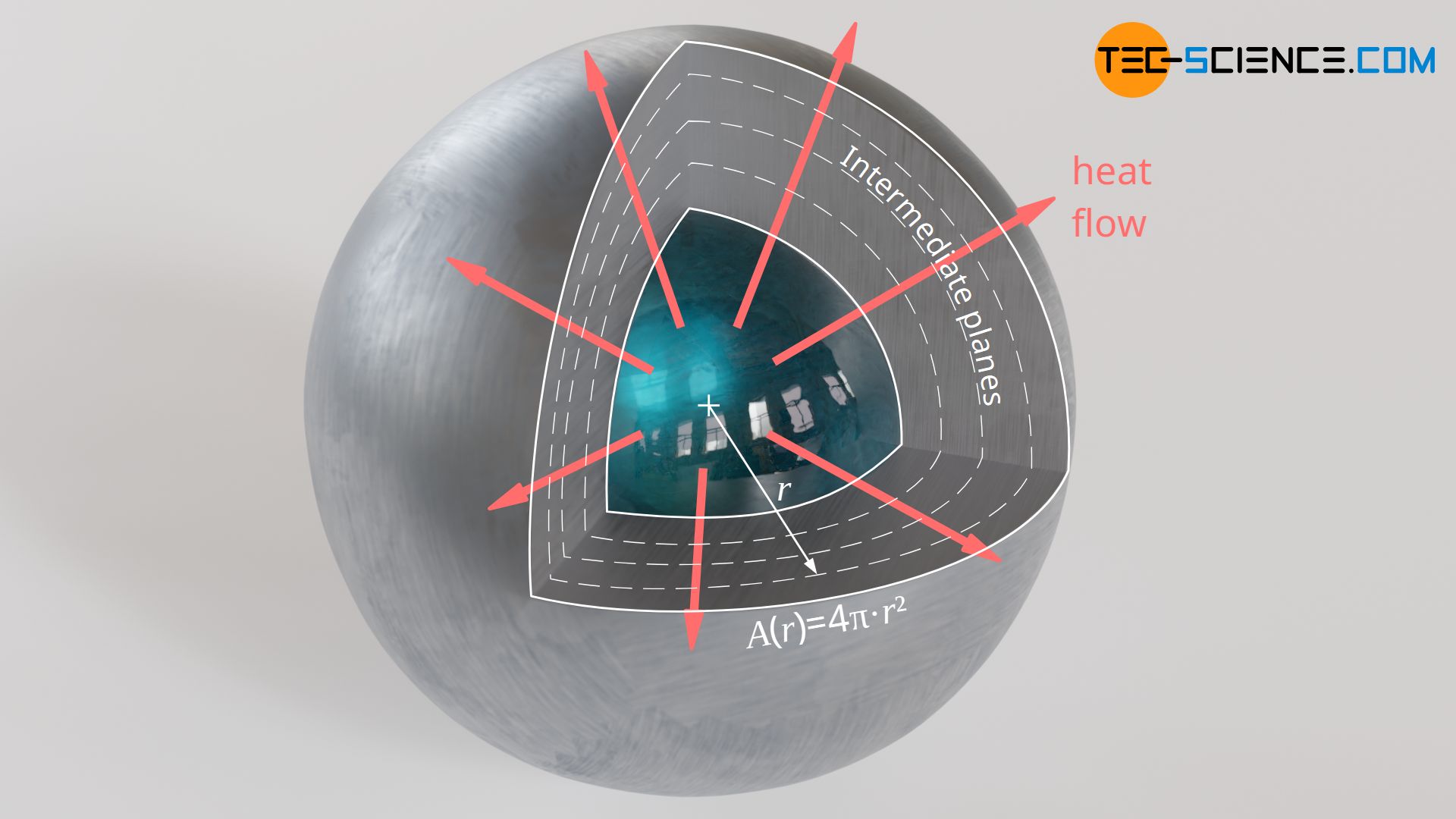
As is the case with a cylindrical pipe, it can therefore be assumed that the temperature changes less and less with increasing radius (flattening of the temperature curve). However, the influence of the radius on the surface area is no longer linear, but quadratic:
\begin{align}
& A(r) = 4\pi \cdot r^2 \\[5px]
\end{align}
After integrating equation (\ref{q}) this finally leads to a hyperbolic temperature profile:
\begin{align}
& \text{d}T = – \frac{\dot Q}{\lambda \cdot A(r)} \cdot \text{d}r \\[5px]
& \int \limits_{T_i}^{T}\text{d}T = – \frac{\dot Q}{\lambda \cdot 4\pi } \cdot \int \limits_{r_i}^{r} \frac{\text{d}r}{r^2} \\[5px]
& [T]_{T_i}^{T}= – \frac{\dot Q}{ \lambda \cdot 4\pi} \cdot \left[-\frac{1}{r}\right]_{r_i}^{r}\\[5px]
& T-T_i= – \frac{\dot Q}{\lambda \cdot 4\pi} \cdot \left(\frac{1}{r_i} -\frac{1}{r} \right)\\[5px]
\label{k}
& \boxed{T(r)= T_i – \frac{\dot Q}{\lambda \cdot 4\pi} \cdot \left(\frac{1}{r_i} -\frac{1}{r} \right) } \\[5px]
\end{align}
The temperature through a spherical wall changes hyperbolically!

Calculation of the heat flows based on the temperatures
Area-specific heat flow through a plane wall
In practice, one is often not so much interested in the temperature curve but rather in the heat flow that one obtains at given temperatures depending on the geometry. In the case of building walls, for example, one is often interested in how much heat per time passes through the walls to the outside when there is a temperature difference. For a plane wall of thickness t this heat flow can be determined by rearranging equation (\ref{e}). With T(r=t) as temperature on the outside To and Ti as temperature on the inside of the wall, the heat flow can be calculated using the following formula:
\begin{align}
& T_o = T_i – \frac{\dot Q}{\lambda \cdot A} \cdot t \\[5px]
\label{ee}
& \underbrace{\frac{\dot Q}{A}}_{\dot q_A} =(T_i-T_o) \cdot \frac{\lambda}{t} \\[5px]
& \boxed{\dot q_A =(T_i-T_o) \cdot \frac{\lambda}{t}} \\[5px]
\end{align}
The quotient of heat flow and area denotes the so-called area-specific heat flow q*A (heat flux). This quotient indicates the heat flow per unit area.
By rearranging equation (\ref{ee}) to form the term Q*/(A⋅λ) and putting it into equation (\ref{z}), one obtains the course of the temperature as a function of the outside temperature To and inside temperature Ti. The temperature curve is therefore independent of the heat flow, the thermal conductivity and the surface area (of course the temperature profile cannot depend on these quantities, as the linear course is unambiguously determined by the inside and outside temperature)!
\begin{align}
& \frac{\dot Q}{A \cdot \lambda} = \frac{T_i-T_o}{t} ~~~~~\text{used in}~~~~~ T(r) = T_i – \frac{\dot Q}{\lambda \cdot A} \cdot r ~\text{:}\\[5px]
&\boxed{T(r) = T_i – \frac{T_i-T_o}{t} \cdot r} \\[5px]
\end{align}
Length-specific heat flow through a cylindrical pipe
In practice, the heat flow of a cylindrical tube is also often of interest rather than the temperature profiles that result. Just imagine the radiator already mentioned. Warm water flows inside the pipe, which is heated to a certain temperature. From the temperature difference between the outside and inside of the radiator, the heat transferred to the air in the room can be determined by rearranging equation (\ref{z}). With T(r=ro) as the temperature on the outside of the radiator (T0) and Ti as the temperature on the inside (water temperature), the heat flow can be calculated using the following formula:
\begin{align}
& T_o = T_i – \frac{\dot Q}{\lambda \cdot 2\pi \cdot l} \cdot \ln\left( \frac{r_o}{r_i}\right) \\[5px]
\label{zz}
&\underbrace{\frac{\dot Q}{l}}_{\dot q_L}= (T_i-T_o) \cdot \frac{ 2 \pi \lambda }{\ln\left( \frac{r_o}{r_i}\right) } \\[5px]
&\boxed{\dot q_L= (T_i – T_o) \cdot \frac{ 2 \pi \lambda }{\ln\left( \frac{r_o}{r_i}\right) }} \\[5px]
\end{align}
The quotient of heat flow and pipe length denotes the so-called length-specific heat flow q*L. This quantity indicates the heat flow per unit length of the pipe.
By rearranging equation (\ref{zz}) to form the term Q*/(2⋅π⋅l⋅λ) and then putting that term into equation (\ref{e}), one obtains the course of the temperature as a function of the outside temperature To and the inside temperature Ti:
\begin{align}
& \frac{\dot Q}{ 2 \pi l \lambda } = \frac{T_i-T_o}{ \ln\left( \frac{r_o}{r_i}\right) } ~~~~~\text{used in}~~~~~ T(r)= T_i – \frac{\dot Q}{2\pi l \lambda } \cdot \ln\left( \frac{r}{r_i}\right) ~\text{:}\\[5px]
&\boxed{T(r) = T_i – \frac{T_i-T_o}{ \ln\left( \frac{r_o}{r_i}\right) } \cdot \ln\left( \frac{r}{r_i}\right) } \\[5px]
\end{align}
Solid-angle-specific heat flow through a hollow sphere
The heat flow through a hollow sphere at a given interior and exterior temperature is determined by rearranging equation (\ref{k}):
\begin{align}
& T_o= T_i – \frac{\dot Q}{\lambda \cdot 4\pi} \cdot \left(\frac{1}{r_i} -\frac{1}{r_o} \right) \\[5px]
\label{kk}
& \frac{\dot Q}{4\pi} = (T_i-T_o) \cdot \frac{\lambda}{ \frac{1}{r_i} -\frac{1}{r_o} } \\[5px]
& \underbrace{\frac{\dot Q}{4\pi}}_{\dot q_S} = (T_i-T_o) \cdot \lambda \cdot \frac{ r_o \cdot r_i}{ r_o -r_i} \\[5px]
& \boxed{ \dot q_S = (T_i-T_o) \cdot \lambda \cdot \frac{ r_o \cdot r_i}{ r_o -r_i}} \\[5px]
\end{align}
The quotient of heat flow and 4π denotes the so-called solid-angle-specific heat flow \q*S. This quantity indicates the heat flow per unit solid angle. For a complete sphere the solid angle is 4π and for a hemisphere 2π.
The following formula applies to the course of the temperature after rearranging equation (\ref{kk}) and then putting it into the equation (\ref{k}):
\begin{align}
& \frac{\dot Q}{ 4 \pi \lambda } = \frac{ T_i-T_o }{ \frac{1}{r_i} -\frac{1}{r_o} } ~~~~~\text{used in}~~~~~ T(r)= T_i – \frac{\dot Q}{4\pi \lambda } \cdot \left(\frac{1}{r_i} -\frac{1}{r} \right) ~\text{:}\\[5px]
&\boxed{T(r) = T_i – \frac{ T_i-T_o }{ \frac{1}{r_i} -\frac{1}{r_o} } \cdot \left(\frac{1}{r_i} -\frac{1}{r} \right) } \\[5px]
\end{align}
Calculation of the heat flow using the mean area
One can reduce the calculation of the heat flow through the geometries described above to a common formula by using the so-called mean area A:
\begin{align}
&\boxed{\dot Q = – \lambda \cdot \bar A \cdot \frac{\text{d}T}{\text{d}r}} \\[5px]
\end{align}
Depending on the geometry, the mean area is calculated as follows:
\begin{align}
&\bar A_{\text{ plane wall}} = A_i = A_o \\[5px]
&\bar A_{\text{ hollow cylinder}} = \frac{A_o-A_i}{\ln\left(\frac{A_o}{A_i}\right)} \\[5px]
&\bar A_{\text{ hollow sphere}} = \sqrt{A_i \cdot A_o} \\[5px]
\end{align}
The area Ai denotes the surface area on the inside of the geometry and Ao the surface area on the outside of the geometry.
")


")

