The viscosity of ideal gases is mainly based on the momentum transfer due to diffusion between the fluid layers.
Definition of viscosity
In the article Viscosity, the cause of viscosity was mainly attributed to attractive forces between the layers of a fluid. These forces act similar to frictional forces, so that the individual fluid layers try to slow each other down. For the definition of viscosity one can imagine a fluid between two plates. The lower plate is at rest and the upper plate is moved at constant speed.
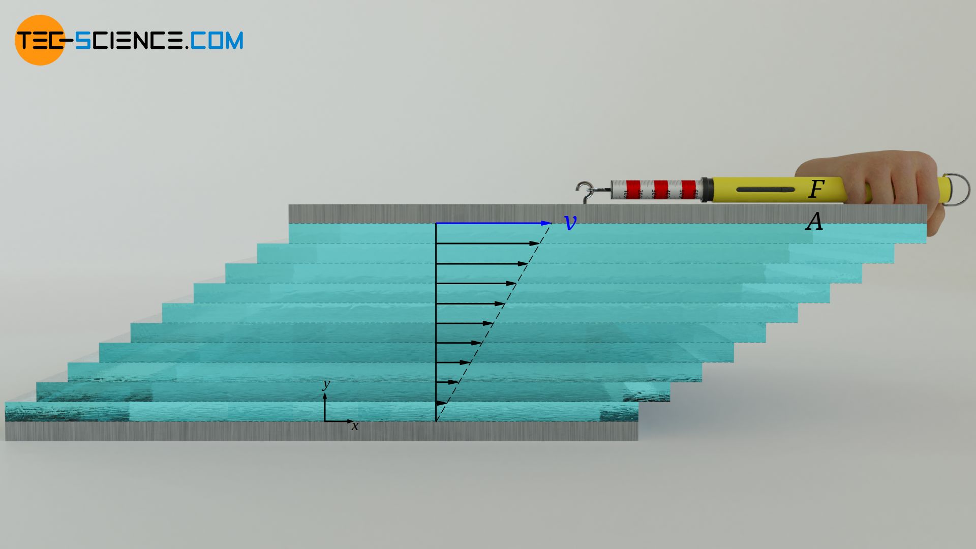
Due to the no-slip condition, both the upper and the lower fluid layer adhere to these plates. The lower fluid layer thus remains at rest and the upper fluid layer moves at the same speed as the upper plate. A linear velocity profile is formed between the plates. A considered fluid layer thus always moves slower than the fluid layer above it. Due to the molecular forces between the molecules, a lower fluid layer always tries to slow down the fluid layer above.
These frictional forces between the layers must be compensated if the uppermost layer is to be moved at a constant speed. The more viscous a fluid is, the stronger the internal friction forces and the greater the force required to move the top plate. The viscosity η shows the relationship between the area-related force F/A (called shear stress τ), which is required to move the fluid layers, and the slope of the velocity profile dv/dy (called velocity gradient):
\begin{align}
\label{t}
&\frac{F}{A}=\boxed{\tau= \eta \cdot \frac{\text{d} v}{\text{d} y}} ~~~~~\text{Newton’s law of fluid friction}\\[5px]
\end{align}
Viscosity of gases (momentum transfer)
The cause of viscosity due to frictional forces acting between the fluid layers can be clearly understood for liquids. In gases, however, the molecules exert almost no molecular forces on each other. Frictional forces between the fluid layers due to intermolecular cohesion are therefore almost non-existent. However, practice shows that even gases have a considerable viscosity and that fluid layers are slowed down in flows. How can this behavior be explained without the presence of inter-molecular forces?
The slowing down effect of fluid layers in gases is mainly due to the momentum transfer of the gas molecules when they diffuse from a slower layer into a faster layer. This process also takes place in liquids, but it is negligible compared to the decelerating effect due to the intermolecular forces.
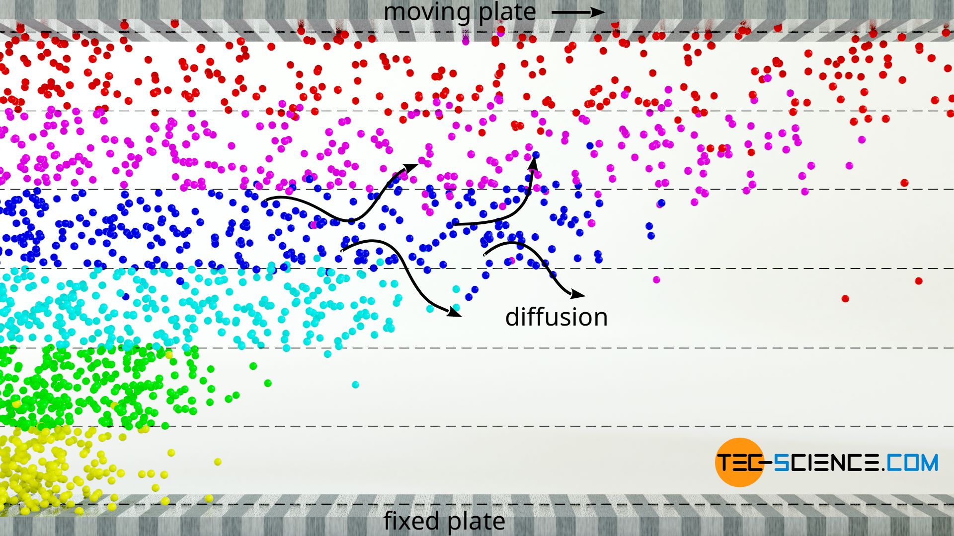
Let us again consider the already mentioned laminar flow, which this time consists of an ideal gas as fluid. If one gas molecule collides with another, an momentum exchange takes place, i.e. a slower molecule takes up part of the momentum of the faster molecule. However, such a momentum transfer does not only take place within a fluid layer. Due to the random molecular motion (Brownian motion), molecules also diffuse into adjacent fluid layers. What happens if a slower molecule diffuses into a layer of faster particles? The fast molecules are slowed down by this diffused gas molecule and the layer slows down.
One can illustrate the situation with a cart and a ball. The cart is to be moved at a constant speed when suddenly the heavy ball is put in while passing by. The ball represents the slower gas molecule (in this case even stands still), which diffuses into the faster fluid layer (illustrated by the cart). Since the ball has a lower speed than the cart when put in, the ball must be accelerated to the speed of the cart if the speed is to remain constant. This requires a force corresponding to the mass of the ball (force = mass x acceleration). This means that if this force would not be applied, the cart would be slowed down, similar to a frictional force.
The diffusion of gas molecules between the layers of a laminar flow leads to a momentum transfer on which the viscosity of gases is mainly based!
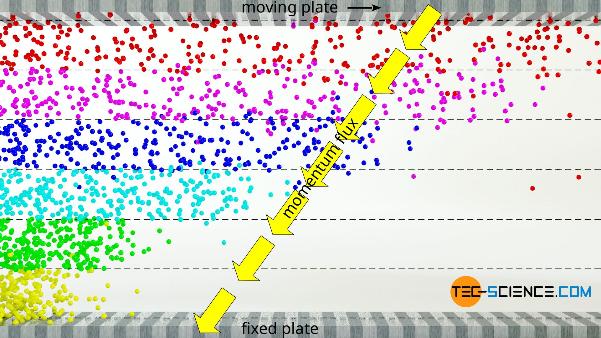
Faster layers thus transfer part of their momentum by diffusion into slower layers. All in all there is a transport of momentum from the moving plate at the top of the fluid to the resting plate at the bottom of the fluid. This momentum transport (which ultimately corresponds to a force between the layers) is directed in the direction of decreasing velocity, so to speak, i.e. against the velocity gradient. The transport of momentum becomes particularly clear when the upper plate is set in motion from rest. First, only the layer directly adhering to the upper plate is set in motion. By the transport of momentum onto the layer underneath, this layer starts to move, etc. The momentum thus gradually spreads through the layers, so to speak.
The resistance that one experiences when moving the upper plate is caused by the fact that the movement of the gas layers is hindered because the lower plate is fixed. Holding the bottom plate in place ultimately requires the same force as maintaining the movement of the upper plate. The momentum is, so to speak, introduced at the upper plate and is transferred from layer to layer and exits at the lower plate. Finally, in a state of equilibrium, there is no net momentum flow, which is transferred to the fluid layers, so that these finally move at constant but different speeds according to the linear velocity profile.
Derivation of the viscosity of ideal gases
Shear stress as momentum flux
A force F can generally be determined from the change in momentum per unit time:
\begin{align}
&F= \frac{\text{d} p}{\text{d} t} = \dot p ~~~~~\Rightarrow~~~~~\boxed{\text{force = momentum flow rate}}\\[5px]
\end{align}
The force acting on the individual fluid layers is thus caused by the change in momentum and can therefore also be understood as momentum flow rate p*. If one relates the force and thus the momentum flow rate to the surface area, this corresponds to a shear stress, which in turn can be interpreted as momentum flux p*A (change in momentum per unit time and unit area):
\begin{align}
&\tau = \frac{F}{A}= \frac{\dot p}{A} = \dot p_\text{A} ~~~~~\Rightarrow~~~~~\boxed{\text{shear stress = momentum flux}}\\[5px]
\end{align}
Newton’s law of fluid friction (\ref{t}) can thus also be represented as follows:
\begin{align}
\label{tt}
&\boxed{\dot p_\text{A} = – \eta \cdot \frac{\text{d} v}{\text{d} y}} \\[5px]
\end{align}
The negative sign was introduced to account for the fact that the momentum flux is transferred away from faster layers to slower layers, i.e. in the direction of decreasing velocity gradient. At this point an interesting analogy can be drawn to other transport mechanisms like heat transport and mass transport, which are ultimately described in a similar way:
| heat transport | mass transport | momentum transport | |
|---|---|---|---|
| law of | Fourier | Fick | Newton |
| \begin{align} \notag &\boxed{\dot q = – \lambda ~\frac{\text{d}T}{\text{d}y}} \end{align} | \begin{align} \notag &\boxed{\dot n = – D~ \frac{\text{d}c}{\text{d}y}} \end{align} | \begin{align} \notag &\boxed{\dot p_a=- \eta~ \frac{\text{d}v}{\text{d}y}} \end{align} | |
| drive | temperature gradient | concentration gradient | velocity gradient |
| characteristic quantity | thermal conductivity | diffusion coefficient | viscosity |
| flux | heat flux | diffusion flux | momentum flux |
Momentum transfer between the layers
With the help of the kinetic theory of gases, the viscosity of ideal gases can be calculated. To derive a formula, we consider a laminar flow, where an ideal gas is placed between two plates. The lower plate is fixed and the upper plate moves with a constant speed.
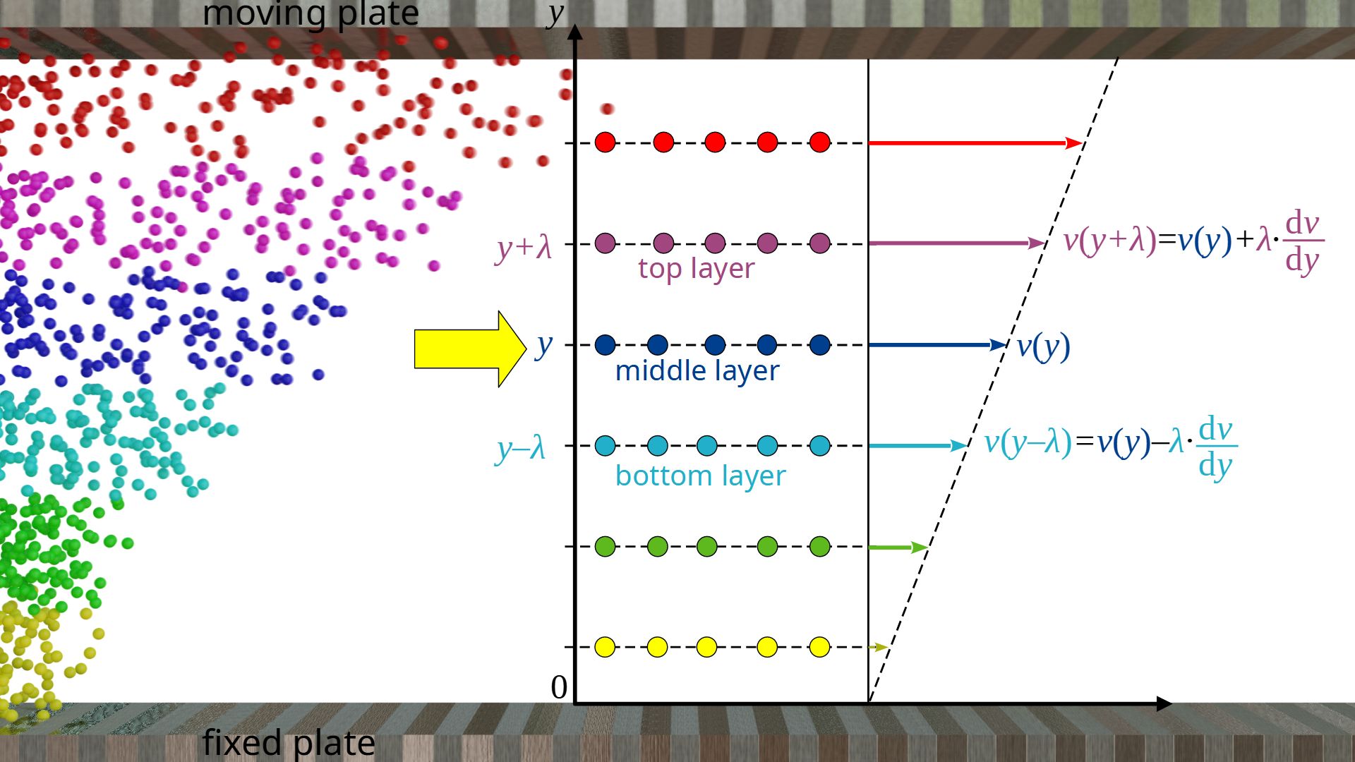
We observe the gas flow on a microscopic level and move along with a fluid layer. The mean distance a gas molecule travels between two collisions is called mean free path λ. We therefore consider gas layers that have a distance λ from each other, so that diffusion processes result in a collision inside those layers and thus in a momentum transfer. We now look at a layer at any height y. The mean velocity of the gas molecules in x-direction with respect to a coordinate system fixed at the resting plate is denoted by vx(y).
The mean velocityvx(y+λ) of the gas molecules in the layer above at the distance λ can be determined using the velocity gradient dv/dy:
\begin{align}
&v_{x}(y+\lambda)= v_{x}(y) + \lambda \cdot \frac{\text{d}v}{\text{d}y} \\[5px]
\end{align}
In the same way, the mean velocity vx(y-λ) of the gas particles in the layer below at the distance λ can be determined:
\begin{align}
&v_{x}(y-\lambda)= v_{x}(y) – \lambda \cdot \frac{\text{d}v}{\text{d}y} \\[5px]
\end{align}
If n*A denotes the particle flux, i.e. the number of particles per unit time and unit area that diffuse from the upper layer or lower layer into the middle layer, then the respective momentum fluxes can be determined with the following formulas. Note that the particle flux is identical for both layers if we assume an incompressible gas flow where the particle density is the same at every point in the flow.
\begin{align}
&\dot p_{A}(y+\lambda) = \dot n_\text{A} \cdot \overbrace{m \cdot v_{x}(y+\lambda)}^{\text{momentum of one molecule}} = \dot n_\text{A} \cdot m \cdot \left(v_{x}(y) + \lambda \cdot \frac{\text{d}v}{\text{d}y} \right) \\[5px]
&\dot p_{A}(y-\lambda) = \dot n_\text{A} \cdot m \cdot v_{x}(y-\lambda) = \dot n_\text{A} \cdot m \cdot \left(v_{x}(y) – \lambda \cdot \frac{\text{d}v}{\text{d}y} \right) \\[5px]
\end{align}
The net momentum flux p*A(y) in the layer at the height y is finally the sum of both momentum fluxes. According to the chosen coordinate system the bottom-up momentum flux (pointing in positive y direction) corresponds to a positive value and the downward facing momentum flux to a negative value.
\begin{align}
\dot p_\text{A}(y) &= \dot p_{A}(y-\lambda) ~-~ \dot p_{A}(y+\lambda) \\[5px]
&= \dot n_\text{A} \cdot m \cdot \left(v_{x}(y) – \lambda \cdot \frac{\text{d}v}{\text{d}y} \right)- \dot n_\text{A} \cdot m \cdot \left(v_{x}(y) + \lambda \cdot \frac{\text{d}v}{\text{d}y} \right) \\[5px]
&= \dot n_\text{A} \cdot m \cdot \left(v_{x}(y) ~- \lambda \cdot \frac{\text{d}v}{\text{d}y} ~-~ v_{x}(y) ~- \lambda \cdot \frac{\text{d}v}{\text{d}y}\right) \\[5px]
\end{align}
\begin{align}
&\boxed{\dot p_\text{A}= – 2~ \dot n_\text{A} \cdot m \cdot \lambda \cdot \frac{\text{d}v}{\text{d}y}}~~~\text{net momentum flux} \\[5px]
\end{align}
Viscosity of ideal gases as a function of particle flux
According to the above equation, the net momentum flux is obviously no longer a function of the variable y and thus identical in every point of the flow! If one compares this formula with Newton’s law of fluid friction (\ref{tt}), it is apparent that the expression 2⋅n*A⋅m⋅λ obviously corresponds to the viscosity η:
\begin{align}
&\dot p_\text{A} = – \eta \cdot \frac{\text{d} v}{\text{d} y} \\[5px]
&\dot p_\text{A}=- \underbrace{2~ \dot n_\text{A} \cdot m \cdot \lambda}_{\eta} \cdot \frac{\text{d}v}{\text{d}y} \\[5px]
\label{eta}
&\boxed{\eta= 2~ \dot n_\text{A} \cdot m \cdot \lambda} ~~~\text{viscosity of ideal gases}\\[5px]
\end{align}
The viscosity of an (ideal) gas is therefore only dependent on the mass of a gas particle, the mean free path and the particle flux. The area-related particle flow n*A, which diffuses in from a layer above or below, depends in turn on how strongly the gas molecules move due to the random diffusion motion (Brownian motion). This in turn is determined by the temperature.
If the temperature is high, diffusion take place more strongly and more particles diffuse between the layers. Thus, the particle flux is high and so is the momentum transfer. This results in an increasing force, which is necessary to maintain the macroscopic flow (movement of the plate)! The viscosity of gases therefore generally increases with temperature and not decreases as with liquids!
At this point it is also evident that with ideal gases, pressure has no influence on viscosity. Although the particle density and thus the diffusing particle flow increases proportionally with increasing pressure, the mean free path decreases to the same extent. Both effects cancel each other out.
With ideal gases the viscosity is independent of pressure and increases with increasing temperature!
Viscosity of ideal gases as a function of temperature
At this point we would like to explicitly derive the dependence of the viscosity of ideal gases on temperature. For this purpose, a correlation between the particle flux diffusing perpendicular to the flow and the temperature must be found.
For this we move in thoughts with a layer, so that this layer rests relative to us. The gas molecules themselves, however, are by no means at rest on the microscopic level. Due to Brownian motion, they move in all directions in a completely random manner. According to the Maxwell-Boltzmann distribution, the mean speed of a gas particle vT is linked to the temperature T of the gas as follows
\begin{align}
\label{a}
&\boxed{ \overline{v_\text{T}} = \sqrt{\frac{8 k_B T}{\pi m}}} ~~~\text{arithmetic mean speed} \\[5px]
\end{align}
In this equation m denotes the mass of a gas molecule and kB is the Boltzmann constant. Note that the speed vT represents the mean speed relative to the moving fluid layers and does not include the superposition of the macroscopic flow motion. The latter has no influence on the temperature anyway; after all, the temperature of a gas does not depend on whether the gas is at rest or moving.
Let us now consider a directed flow in which all particles move in the same direction with the (mean) velocity v. The number of particles flowing per unit time and area (particle flux) can be determined as follows. We consider an area element dA through which the particles flow with the (mean) velocity v within a time dt. The particles cover the distance dl=v⋅dt. Thus the particles obviously flow through the volume element dV:
\begin{align}
&\text{d}V =\text{d}A \cdot \text{d}l = \text{d}A \cdot \overline{v} \cdot \text{d}t \\[5px]
\end{align}
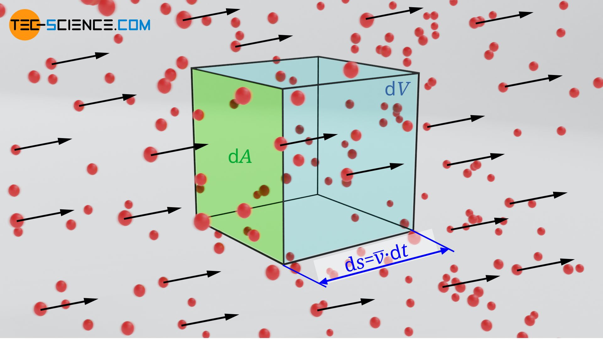
For a given particle density n (number of particles per unit volume), the following number of particles dN will be found this volume element:
\begin{align}
&\text{d}N = n \cdot \text{d}V =n \cdot \text{d}A \cdot \overline{v} \cdot \text{d}t \\[5px]
\end{align}
The number of particles per unit time and area (particle flux n*A) passing through an area perpendicular to the flow can thus be calculated with the following formula:
\begin{align}
&\dot n_\text{A} = \frac{\text{d}N}{\text{d}A \cdot \text{d}t} =n \cdot \overline{v} \\[5px]
&\boxed{\dot n_\text{A} =n \cdot \overline{v} } ~~~\text{particle flux of a directed motion}\\[5px]
\end{align}
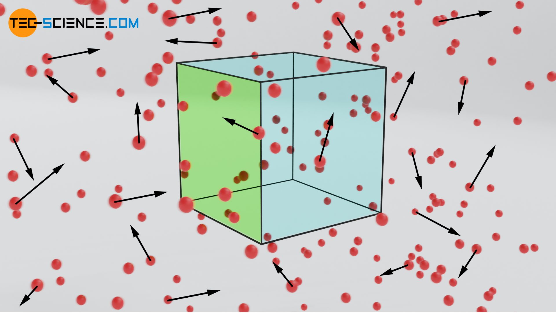
Let us now look again at our laminar flow and we move along in our thoughts with a fluid layer. From this point of view, the flow is no longer directed, but completely random with a mean molecular velocity denoted by vT. The molecules do not move in any preferred direction. This means that only a sixth of the particles move downwards and diffuse into a gas layer below. The particle flux directed perpendicular to the main flow (bulk motion) is thus only one-sixth as large:
\begin{align}
\label{na}
&\boxed{\dot n_\text{A} = \frac{1}{6} n \cdot \overline{v_\text{T}} } ~~~\text{particle flux of a random motion}\\[5px]
\end{align}
Using (\ref{a}) in equation (\ref{na}) results in the following diffusing particle flux as a function of temperature:
\begin{align}
&\dot n_\text{A} = \frac{1}{6} n \cdot \underbrace{\sqrt{\frac{8 k_B T}{\pi m}}}_{\overline{v_\text{T}}} \\[5px]
\end{align}
This equation used in formula (\ref{eta}) finally shows the following relationship between viscosity and temperature:
\begin{align}
&\eta= 2~ \dot n_\text{A} \cdot m \cdot \lambda \\[5px]
&\eta= 2~ \frac{1}{6} n \cdot \sqrt{\frac{8 k_B T}{\pi m}} \cdot m \cdot \lambda \\[5px]
\label{ac}
&\boxed{\eta= \frac{1}{3} n \cdot \sqrt{\frac{8 k_B m T}{\pi}} \cdot \lambda} \\[5px]
\end{align}
Last but not least, the mean free path λ can be expressed by the particle density n and the diameter of the gas molecules d (for the derivation of this formula see article Mean free path & collision frequency):
\begin{align}
& \boxed{\lambda = \frac{1}{\sqrt{2}~n ~\pi d^2}} \\[5px]
\end{align}
Using this formula in equation (\ref{ac}), the following formula for calculating the viscosity of ideal gases is finally obtained:
\begin{align}
&\eta= \frac{1}{3} n \cdot \sqrt{\frac{8 k_B m T}{\pi}} \cdot \lambda \\[5px]
&\eta= \frac{1}{3} n \cdot \sqrt{\frac{8 k_B m T}{\pi}} \cdot \frac{1}{\sqrt{2}~n ~\pi d^2} \\[5px]
&\boxed{\eta= \sqrt{\frac{4 k_B m~T}{9\pi^3~d^4}}} \\[5px]
&\boxed{\eta \sim \sqrt{T}} \\[5px]
\end{align}
This formula shows that the particle density and thus the pressure has no influence on the viscosity of ideal gases. Only the temperature as a variable quantity influences the viscosity. The viscosity increases proportionally with the square root of the temperature!
Note that this formula only applies to laminar flows where the gas layers do not mix macroscopically and diffusion between the layers only occur at the microscopic level. In turbulent flows, the momentum exchange through the turbulence is greater and the viscosity is higher.
Comparing viscosity and thermal conductivity
Equation (\ref{na}) can also be put directly into the formula (\ref{eta}) for the viscosity, resulting in the following relationship:
\begin{align}
&\eta= 2~ \dot n_\text{A} \cdot m \cdot \lambda \\[5px]
&\eta= 2~ \frac{1}{6} n \cdot \overline{v_\text{T}} \cdot m \cdot \lambda \\[5px]
&\eta= \frac{1}{3} \underbrace{n \cdot m}_{\rho} \cdot \lambda \cdot \overline{v_\text{T}} \\[5px]
&\boxed{\eta= \frac{1}{3} \cdot \rho \cdot \lambda \cdot \overline{v_\text{T}}} \\[5px]
\end{align}
This derivation exploited the fact that the product of particle density and mass of a single particle equals the density ϱ of the gas. At this point an interesting analogy to thermal conductivity k of ideal gases can be seen (to avoid confusion with the mean free path, the thermal conductivity was not denoted by λ but k):
\begin{align}
& \boxed{k= \frac{1}{3} \cdot \rho \cdot \lambda \cdot c_v \cdot \overline{v_\text{T}} } \\[5px]
\end{align}
The thermal conductivity thus obeys in principle the same laws as the viscosity, i.e. it increases with increasing mean particle speed (increasing temperature). This is not surprising, since the diffusion of particles is not only associated with an momentum transfer, but also with a energy transfer in terms of heat.
")


")
")
