Viscometry is the experimental determination of the viscosity of liquids and gases with so-called viscometers.
Definition of viscosity (Newton’s law of fluid friction)
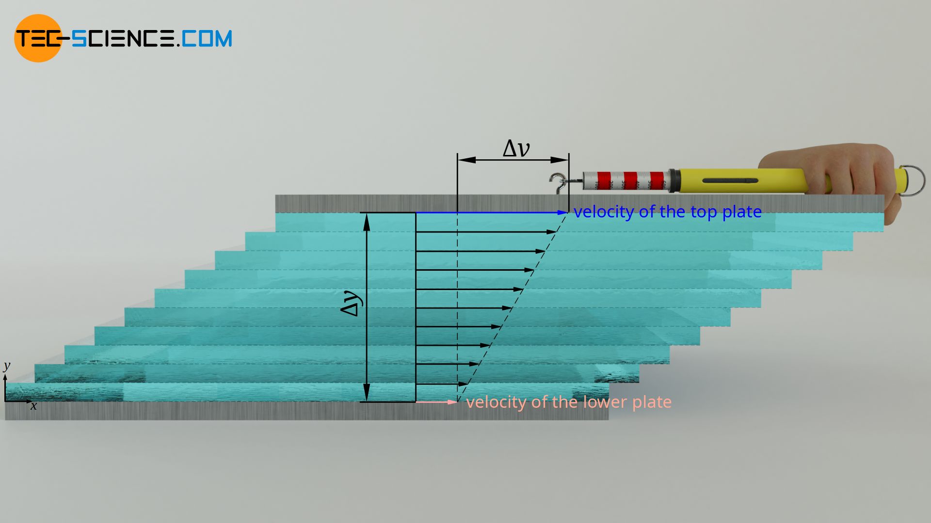
Viscosity describes the internal resistance to flow of a fluid (internal friction). It is defined by the shear stress τ required to shift two plates moving relative to each other. The higher the relative velocity Δv of the plates and the smaller the distance Δy between the plates, the greater the shear stress. The proportionality constant between these quantities is the (dynamic) viscosity η. This law is also known as Newton’s law of fluid friction:
\begin{align}
\label{t}
&\boxed{\tau= \eta \cdot \frac{\Delta v}{\Delta y}} ~~~&&\text{Newton’s law of fluid friction}\\[5px]
&{\tau=\frac{F}{A}} ~~~&&\text{ shear stress} \\[5px]
\end{align}
More detailed information on viscosity and Newton’s law of fluid friction can be found in the article Viscosity.
Rotational viscometer
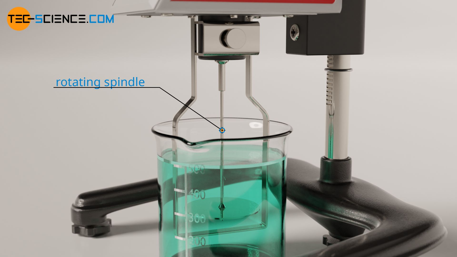
The confinement of a fluid between two plates to define the viscosity is a very descriptive procedure, but is hardly feasible in practice. How should the fluid be held within the gap between two plates? In practice, therefore, a spindle is used which rotates at a constant speed in a cylindrical vessel. The vessel contains the fluid whose viscosity is to be determined. Such an apparatus for determining the viscosity is also called a rotational viscometer.
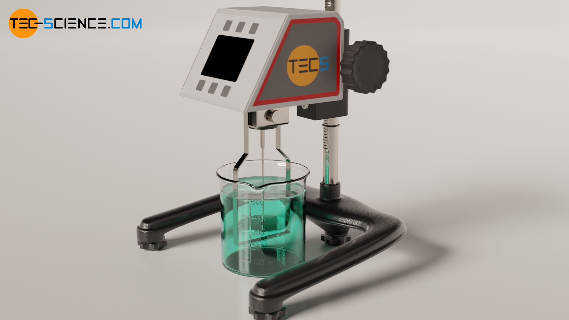
Depending on the viscosity, the drive of the spindle requires a certain torque. The higher the viscosity, the greater the torque required to keep the rotational speed constant. This torque is measured directly at the motor and can be used to determine the viscosity after an appropriate calibration. However, the rotational speed must not be selected too high, because at too high speeds no laminar flow is developed but a turbulent flow.
Falling sphere viscometer
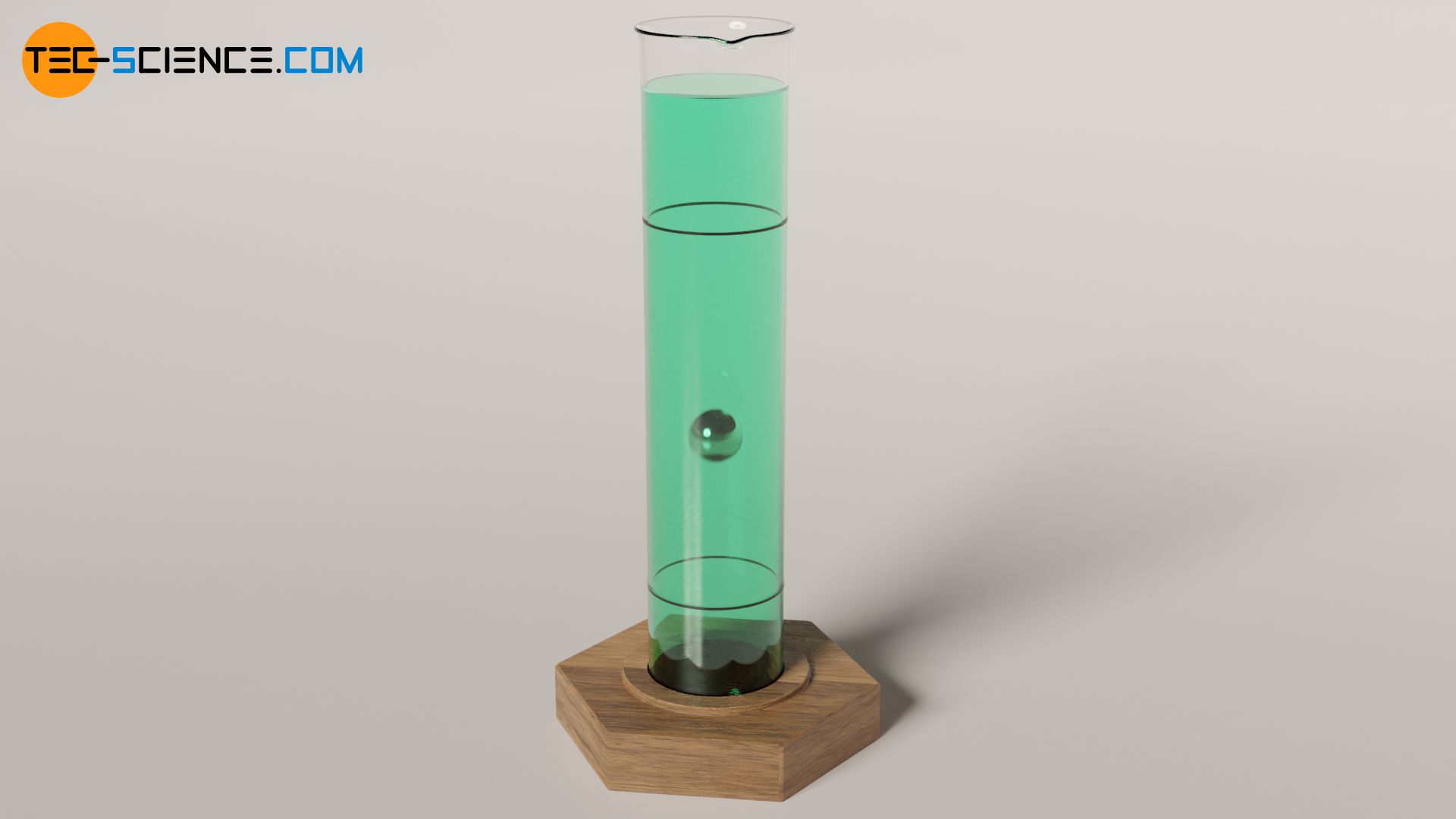
The viscosity of a liquid can also be determined by experiments with a ball sinking into the liquid. The speed at which a ball sinks to the ground in a fluid is directly dependent on the viscosity of the fluid. The fluids used are mainly liquids.
The physicist George Gabriel Stokes derived the following equation, which shows the relationship between the speed v at which a sphere of radius r is drawn through a fluid of viscosity η and the resulting frictional force Ff:
\begin{align}
\label{s}
&\boxed{F_f = 6\pi \cdot r \cdot \eta \cdot v} ~~~\text{Stokes’ law of friction} \\[5px]
\end{align}
Note that Stoke’s law only applies to spherical bodies that are laminar flowed around!
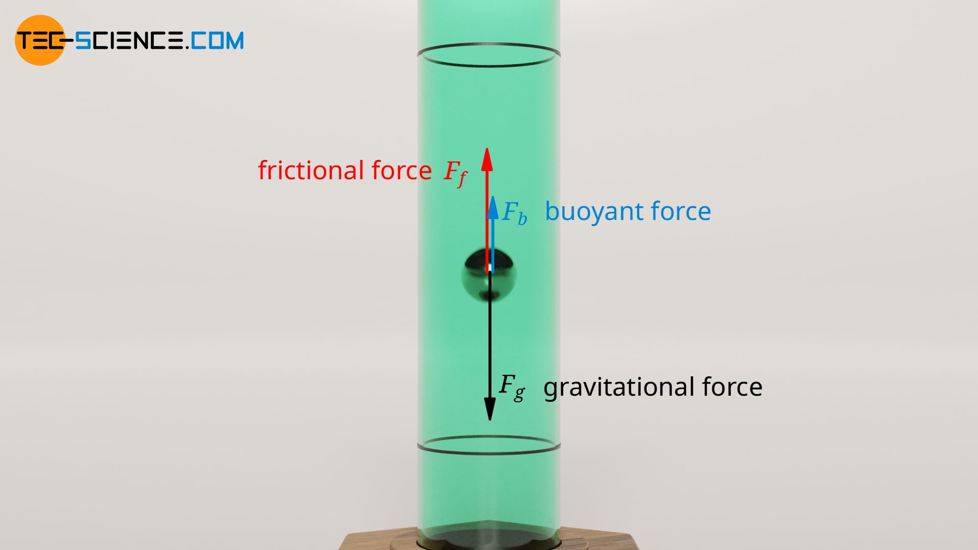
If a ball is dropped in a viscous liquid, the speed increases at first until the opposing frictional force is as great as the weight force of the ball. For more accurate measurements, the upward buoyant force must also be taken into account. All three forces balance each other in the steady case and a constant sinking speed is obtained:
\begin{align}
\label{gg}
&F_g \overset{!}{=} F_f + F_b \\[5px]
\end{align}
The weight force Fg of the ball can be determined via the volume Vb and the density of the ball ϱb:
\begin{align}
\label{g}
&F_g = m_b \cdot g = V_b \cdot \rho_b \cdot g= \frac{4}{3}\pi r^3 \cdot \rho_b \cdot g\\[5px]
\end{align}
The buoyant force Fb is determined on the basis of the Archimedes’ principle from the weight force of the displaced liquid, whereby the displaced volume corresponds exactly to the volume of the ball:
\begin{align}
\label{a}
&F_b = m_f \cdot g = V_b \cdot \rho_f \cdot g= \frac{4}{3}\pi r^3 \cdot \rho_f \cdot g \\[5px]
\end{align}
If one now uses the equations (\ref{s}), (\ref{g}) and (\ref{a}) and put them into equation (\ref{gg}), then the viscosity η of the liquid can be determined from its sinking speed vs:
\begin{align}
&F_g \overset{!}{=} F_f + F_b \\[5px]
&\frac{4}{3}\pi r^3 \cdot \rho_b \cdot g = 6\pi \cdot r \cdot \eta \cdot v_\text{s} + \frac{4}{3}\pi r^3 \cdot \rho_f \cdot g \\[5px]
&6\pi \cdot r \cdot \eta \cdot v_\text{s} = \frac{4}{3}\pi r^3 \cdot \rho_b \cdot g ~- \frac{4}{3}\pi r^3 \cdot \rho_f \cdot g \\[5px]
&6\pi \cdot r \cdot \eta \cdot v_\text{s} = \frac{4}{3}\pi r^3 g \left(\rho_b-\rho_f\right) \\[5px]
\label{e}
&\boxed{\eta = \frac{2r^2g}{9~ v_\text{s}}\left(\rho_b-\rho_f\right) } ~~~~~r \ll R\\[5px]
\end{align}
When performing the experiment, however, the sink rate must not be too high. On the one hand, because then it cannot be ensured that a state of equilibrium has been reached before the ball hits the ground. On the other hand, a laminar flow around the ball must always be assured, which is not the case at high speeds, as turbulence is then created.
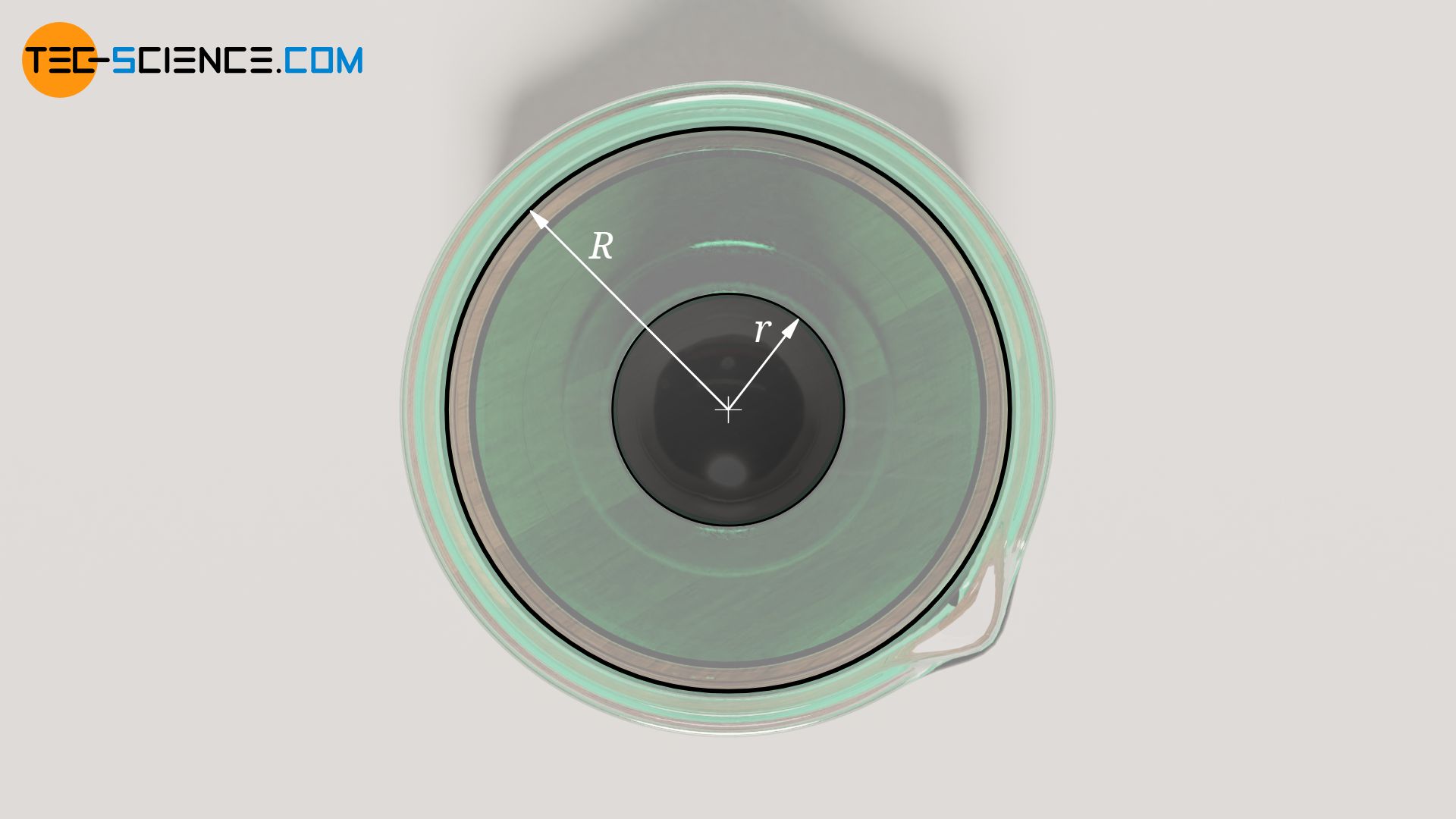
Furthermore, the radius R of the cylindrical tube should be large compared to the radius r of the ball falling within it, otherwise there will be flow effects between the ball and the tube wall that can no longer be neglected. This results in additional friction of the liquid flowing past and a reduction in the sinking speed of the ball (principle of hydraulic damping). Due to the finite radius of the tube, the sinking speed of the ball is therefore always measured too small in practice. Therefore, the sinking velocity is corrected with an empirical correction factor L (called Ladenburg factor):
\begin{align}
\label{h}
&\boxed{\eta = \frac{2r^2g}{9 ~v_\text{s} \cdot L}\left(\rho_b-\rho_f\right) } ~~~\text{where}~~~ \boxed{L=1+2.1 \frac{r}{R}}>1 \\[5px]
\end{align}
In practice, the correction factor is usually determined in advance of the test using a liquid of known viscosity.
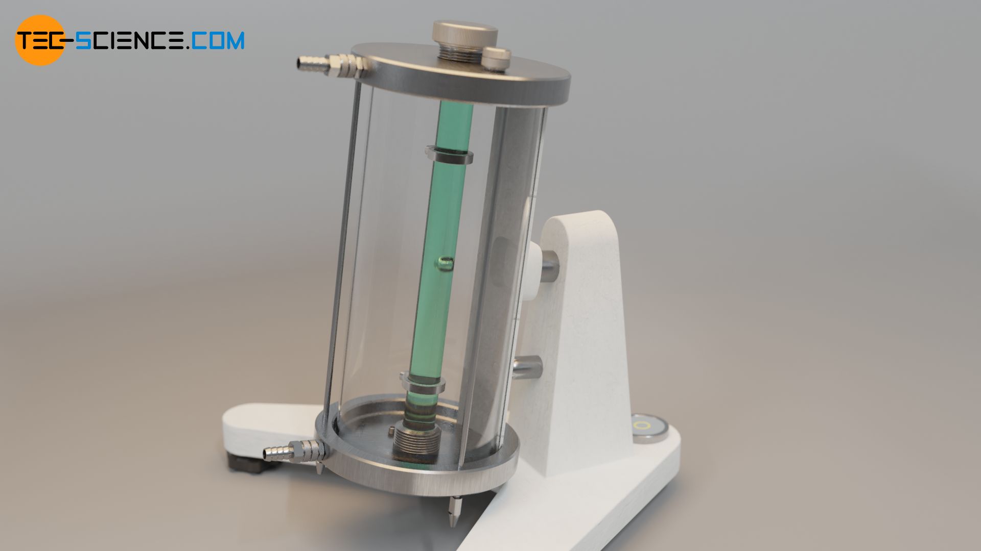
Falling sphere viscometer by Höppler
The falling ball viscometer by Höppler is based on the falling sphere method described in the previous section. A ball falls to the ground in a tube which contains the liquid to be examined. Two markings are attached to the tube which indicate a defined measuring distance Δs (“falling distance”). The time Δt required for the ball to pass through this measuring distance is measured by means of light barriers. The speed of descent vs of the sphere is therefore given by the following formula:
\begin{align}
& v_\text{s} = \frac{\Delta s}{\Delta t}\\[5px]
\end{align}
If the formula for the rate of descent is used in equation (\ref{h}), the viscosity η of the liquid can be determined with the following formula:
\begin{align}
&\eta = \underbrace{\color{red}{\frac{2r^2g}{9 \cdot \Delta s \cdot L}}}_{\text{constant}~ \color{red}{C}} \cdot \left(\rho_b-\rho_f\right) \cdot \Delta t\\[5px]
\label{eta}
&\boxed{\eta = C \cdot \left(\rho_b-\rho_f\right) \cdot \Delta t } \\[5px]\\[5px]
\end{align}
The term marked in red is a specific constant of the measuring apparatus, which also depends on the test sphere used. Depending on the viscosity to be expected, the manufacturers of Höppler viscometers provide various balls for which the test constant C has been determined in advance.
This constant also takes into account that the tube is not exactly vertical, but inclined. Therefore the ball sinks not only by falling, but also by rolling. This rolling motion guides the test ball stably downwards. In this way, turbulence in the liquid is avoided and the validity of Stokes’ Law is ensured, i.e. in particular the proportionality between frictional force and sinking speed. In the case of turbulent flow, the frictional force would no longer be proportional to the sinking speed and the viscosity would no longer be a linear function of the duration of the fall – equation (\ref{eta}) would no longer be valid.
In order to study the temperature influence on the viscosity, the tube is usually placed in another tube filled with water. Circulating thermostats can be used to precisely control the temperature of the water bath and thus the liquid to be examined.
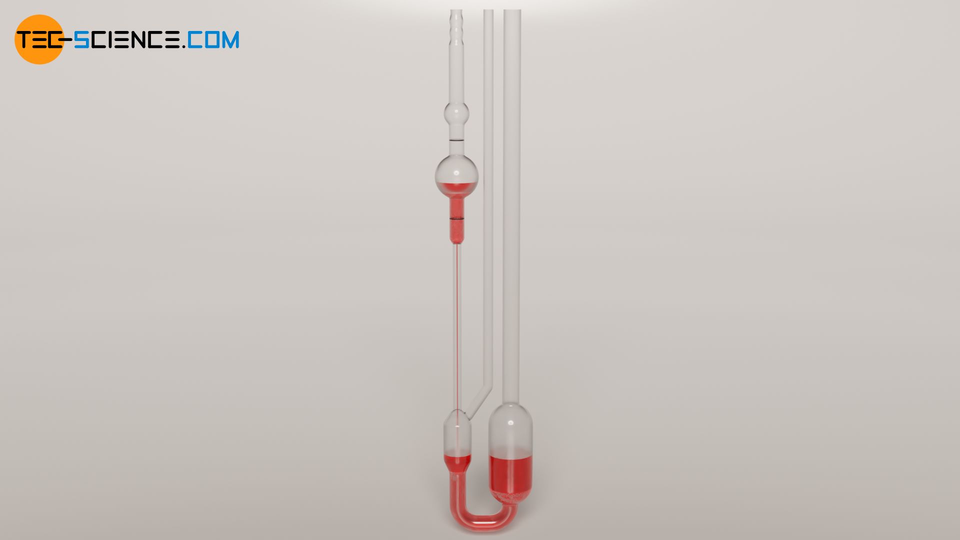
Capillary viscometer by Ubbelohde
The capillary viscometer is based on the Hagen-Poiseuille law for pipe flows. This law states that the volumetric flow rate V* through a capillary is dependent on the viscosity η of the liquid flowing through (assumed that the flow is fully developed):
\begin{align}
&\boxed{\dot V = – \frac{\pi R^4}{8 l \eta}\Delta p } \\[5px]
\end{align}
In this equation, R denotes the radius of the capillary and l its length. The pressure difference Δp corresponds to the pressure drop between the beginning and end of the capillary, which ultimately causes the flow of the liquid. Below the capillary is an L-shaped tube so that the same ambient pressure applies above and below the capillary. Thus the liquid is driven only by the hydrostatic pressure. The pressure drop Δp is thus dependent on the density of the liquid.
The volumetric flow rate through the capillary can be determined by measuring time and mass that has flowed through. However, manufacturers of capillary viscometers usually summarize the device-dependent variables such as radius and length of the capillary in a constant C. Thus, only the time period t has to be determined within which the liquid in the reservoir has passed two marks. In addition, the density of the fluid ϱf is required, since this determines the pressure drop in the Hagen-Poiseuille law. With the following formula the viscosity η can then be determined:
\begin{align}
&\boxed{\eta= C \cdot \rho_f \cdot (t-t_c)} \\[5px]
\end{align}
As already mentioned, the Hagen-Poiseuille law only applies to a fully developed flow. At transition from reservoir to capillary (and up to some degree also within the capillary) however, the flow is not yet fully developed, but is accelerated. The energy required to accelerate the fluid means an additional pressure drop. To take this into account, the measured time is therefore corrected by a so-called Hagenbach correction time tc.
Dip cup viscometer
A very simple method for determining viscosity is the dip cup viscometer. This method makes use of the fact that the discharge of a liquid through a hole in a vessel also depends on the viscosity. Due to the high flow resistance, highly viscous liquids take a relatively long time to flow out through a hole in the dip cup. For a given cup volume, the time required to discharge the liquid is therefore a direct measure of viscosity.
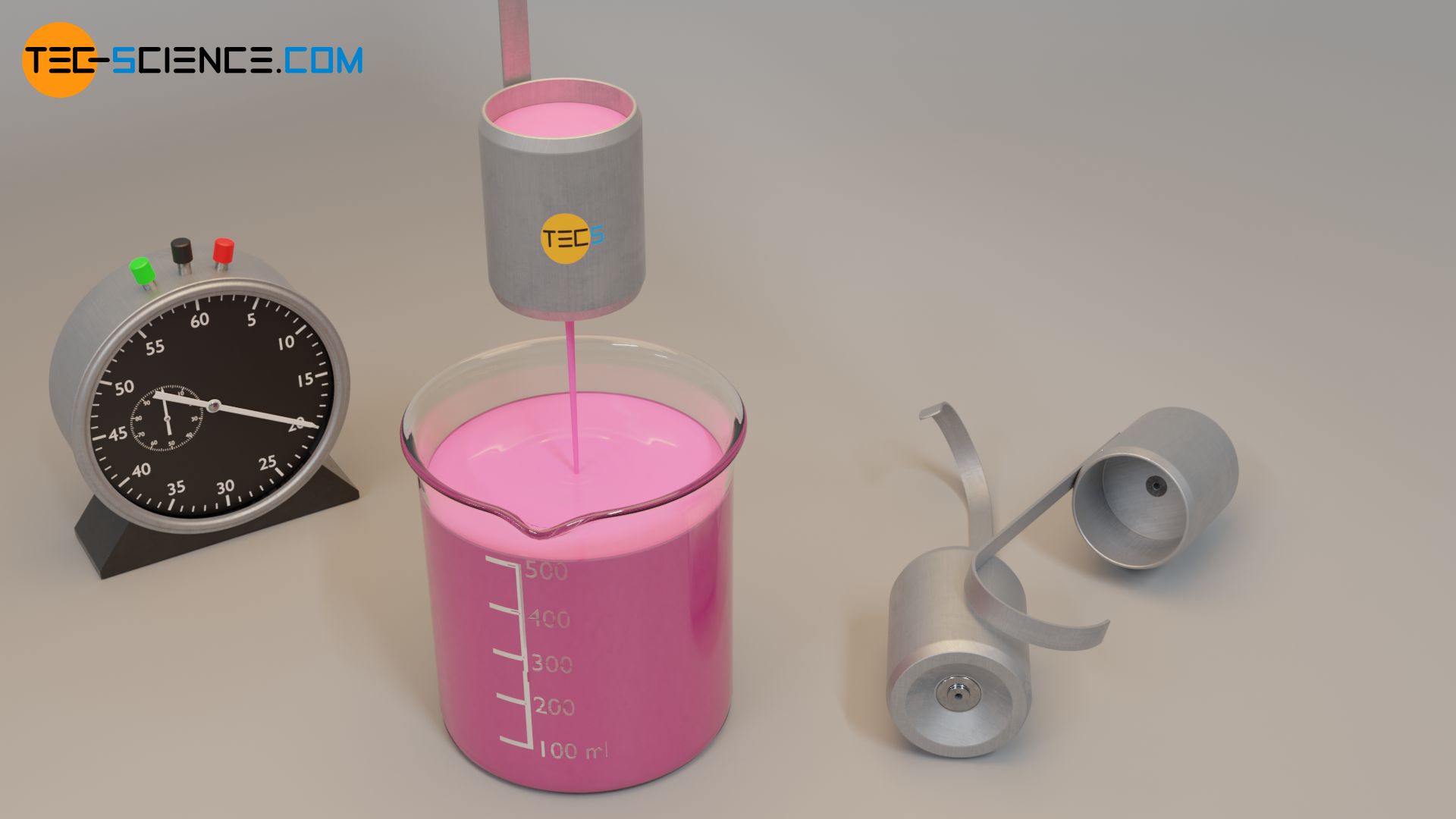
Manufacturers of dip cups list the corresponding viscosity in their data sheets depending on the discharge time. Depending on the viscosity to be expected, different dip cups are to be used. In order to obtain valid results, the discharge time must also be within a certain range. If this is not the case, another dip cup must be used.
The dip cup viscosimeter is mainly used to determine the viscosity of paints or lacquers. These liquids would otherwise heavily contaminate conventional viscometers. Furthermore, very fast results are obtained with a dip cup viscometer, so that paints or lacquers can be checked and further processed immediately after mixing.
")


")
")
