Derivation of the barometric formula (adiabatic atmosphere)

The barometric formula for an adiabatic atmosphere takes into account the decrease in temperature with increasing altitude and the associated effects on air pressure.

Barometric formula for an isothermal atmosphere

In the article Barometric formula for an isothermal atmosphere the barometric formula was derived in detail under the assumption of a constant temperature. Therefore, only a short version of the derivation will be given here.

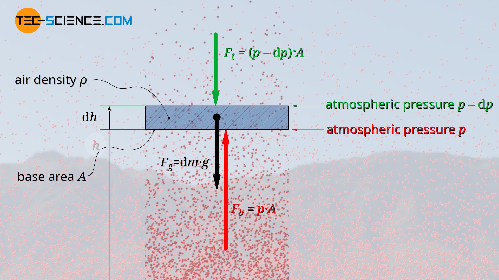
A layer of air (called air parcel) with the infinitesimal thickness dh, which is in equilibrium with the environment, is considered. This air parcel is located at an arbitrary altitude h at which the air density is ϱ. In this case one is dealing with three forces which are all in equilibrium. Firstly, a pressure p acts on the bottom side of the air layer. On the other hand, due to the decreasing air density, a low air pressure acts on the top side. The pressure there is lower by an amount dp. The corresponding forces on both sides of the air parcel can be determined by the product of pressure and base area A. The third force is the weight F_g of the air parcel.

\begin{align}
F_b &= p \cdot A &\text{force at the bottom of the air layer} \\[5px]
F_t &= \left(p-\text{d} p \right) \cdot A &\text{force at the top of the air layer } \\[5px]
F_g&= A \cdot \text{d} h \cdot \rho \cdot g &\text{weight of the air layer} \\[5px]
\end{align}

The downwards directed force of the air pressure on the top side of the air layer F_t and the weight F_g also acting downwards are thus in balance with the upwards directed force on the bottom side of the air layer F_b.

\begin{align}
\require{cancel}
& F_b \overset{!}{=} F_g + F_t \\[5px]
& p \cdot \bcancel{A} = \bcancel{A} \cdot \text{d}h \cdot \rho \cdot g + \left(p-\text{d}p \right) \cdot \bcancel{A} \\[5px]
&\bcancel{p} = \text{d}h \cdot \rho \cdot g + \bcancel{p} – \text{d}p \\[5px]
&\text{d}p = \rho \cdot g \cdot \text{d}h \\[5px]
\end{align}

To take into account the fact that the pressure decreases with increasing altitude (dh>0) and does not increase (dp<0), a negativ sign is added to the equation above:

\begin{align}
\label{dp}
&\boxed{\text{d}p =- \rho \cdot g \cdot \text{d}h} \\[5px]
\end{align}

This equation thus shows the relationship between an (infinitesimal) change in altitude dh and the resulting (infinitesimal) change in pressure dp. However, the fact that the air density itself is a function of pressure is somewhat disturbing at this point. For the higher the pressure, the more compressed the air is and the denser it is. It is therefore necessary to express density as a function of pressure. This is relatively easy to do if you consider air to be an ideal gas. According to the ideal gas law, density is related to pressure by the temperature T (where R_s denotes the specific gas constant):

\begin{align}
\label{ideal}
&p=R_s \cdot \rho \cdot T~~~~~\text{ideal gas law} \\[5px]
\label{rho}
&\boxed{\rho=\frac{p}{ R_s \cdot T }}\\[5px]
\end{align}

If equation (\ref{rho}) is used in equation (\ref{dp}), the following relationship is finally obtained between an (infinitesimal) change in altitude and the resulting change in pressure:

\begin{align}
\label{c}
&\boxed{\text{d}p = -\frac{g}{R_s \cdot T} \cdot p \cdot \text{d} h} \\[5px]
\end{align}

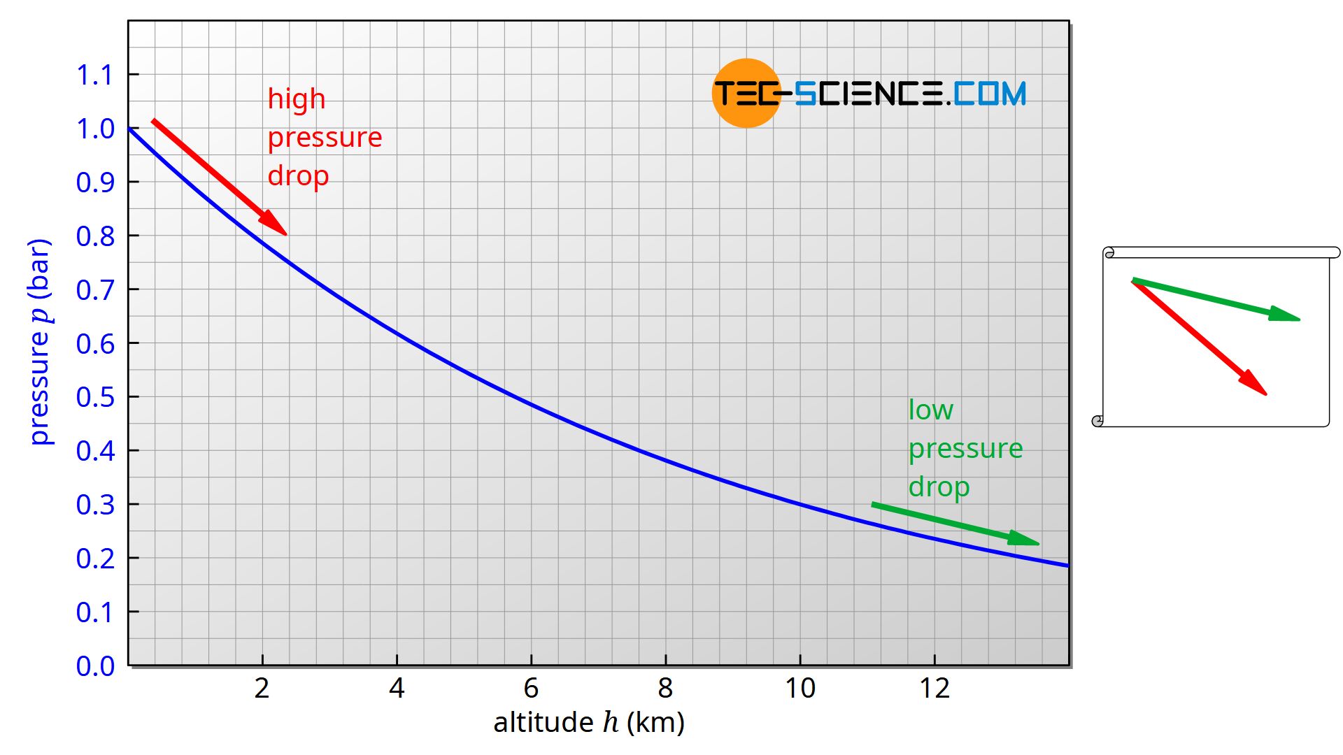
It is now immediately apparent that the pressure change is directly influenced by the pressure itself. The lower the pressure, the smaller the pressure change will be (assuming the same change in altitude dh. It can therefore be assumed that the air pressure will decrease less with increasing altitude. If one represents the decrease in pressure over altitude, one consequently obtains a curve that becomes increasingly flatter. As the pressure change is proportional to the pressure, an exponential decrease in pressure is obtained.

One obtains this curve by integrating equation (\ref{c}) after separating the variables. The integration assumes a constant temperature. The result is the classical barometric formula (see the linked article for a detailed derivation with more explanations):

\begin{align}
&\text{d}p = -\frac{g}{R_s \cdot T} \cdot p \cdot \text{d} h \\[5px]
&\frac{ \text{d}p }{p} = -\frac{g}{R_s \cdot T} \cdot p \cdot \text{d} h \\[5px]
&\int_{p_0}^{p}\frac{ \text{d}p }{p} =-\frac{g}{R_s \cdot T} \cdot \int_{0}^h \text{d} h \\[5px]
&\left[\ln{\left( p\right)}\right]_{p_0}^p = -\frac{g}{R_s \cdot T} \cdot \left[~h~\right]_{0}^{h}\\[5px]
& \ln{(p)}-\ln{(p_0)}= -\frac{g}{R_s \cdot T} \cdot {\left(h-0\right)}\\[5px]
& \ln{\left(\frac{p}{p_0}\right)}= -\frac{g \cdot h}{R_s \cdot T} \\[5px]
& \text{e}^{\Large{\ln{\left(\frac{p}{p_0}\right)}}}= \text{e}^{\Large{-\frac{g \cdot h}{R_s \cdot T} }}\\[5px]
&\frac{p}{p_0}= \text{e}^{-\frac{g \cdot h}{R_s \cdot T} }\\[5px]
\label{bar}
&\boxed{p(h)= p_0 \cdot \text{e}^{\Large{-\frac{g \cdot h}{R_s \cdot T}}}} ~~~~~\text{barometric formula for an isothermal atmosphere} \\[5px]
\end{align}

In this equation, p₀ denotes the pressure at the reference level (“zero height”) and p corresponds to the pressure at any height h above the reference level.

Influence of a temperature change on the barometric formula (adiabatic atmosphere)

As already mentioned, the barometric formula according to the equation (\ref{bar}) was derived with the condition of a constant temperature. This formula is therefore only valid if it is assumed that the temperature of the atmosphere does not change with altitude. In this context one speaks of a so-called isothermal atmosphere.

The “classical” barometric formula only applies to an isothermal atmosphere, i.e. under the condition that the temperature does not change with increasing altitude.

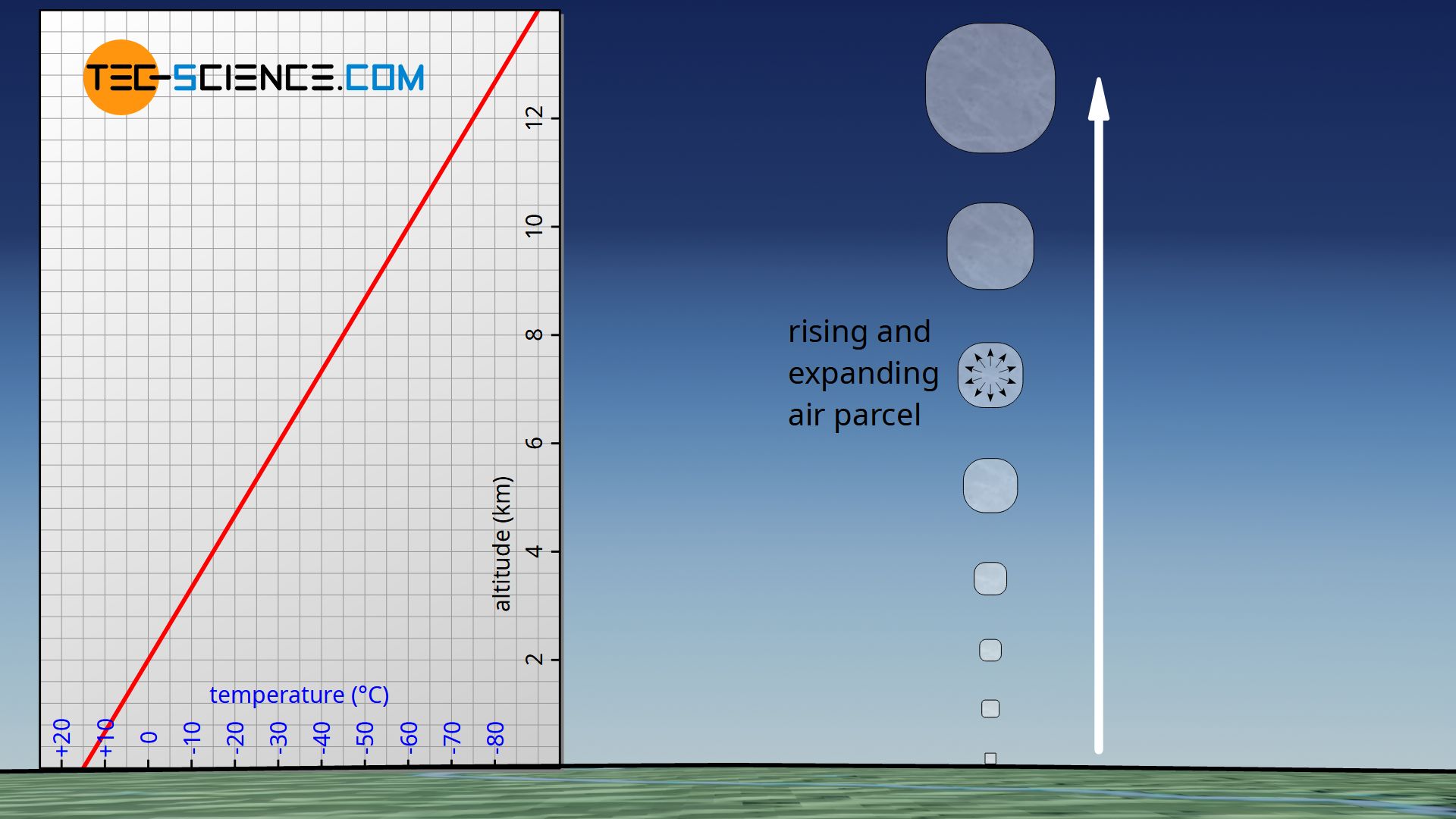
However, especially when considering large changes in altitude, practice shows that the temperature does not remain constant, but usually decreases with increasing altitude. For this reason, it is generally colder on high mountains than in the surrounding valleys. This can be attributed, among other things, to the fact that warm air that rises to the top due to thermals cools down due to the decreasing pressure. Such a phenomenon can also be observed with spray cans. The pressurized gas will cool down considerably when it expands into the surrounding, i.e. when it is expanded to a lower pressure.

For a more precise description of the pressure profile, one must therefore take into account the change in temperature. In order to model the temperature change, we will consider an air parcel in the following, which rises and expands due to the decreasing pressure and cools down as a result. For simplicity, it is assumed that the air parcel does not give off any heat to the environment and does not absorb any from it. It is therefore an adiabatic system. In this context, one also speaks of a so-called adiabatic atmosphere.

Relationship between change in altitude and change in temperature (lapse rate)

Note that just because no heat is transferred during an adiabatic change of state does not mean that the temperature does not change. In this case, the temperature change is only due to the change in pressure or volume during the rising and not to external heat transfer, which simplifies the modelling accordingly.

For the air parcel considered to be an adiabatic system, one must therefore first find a relationship between a change in pressure (which is linked to the change in altitude) and the resulting change in temperature. In this way, the temperature decrease can be described mathematically and then incorporated into the barometric formula.

For this purpose, the first law of thermodynamics in differential notation is necessary. This equation states in that an (infinitesimal) supply of work dW and heat dQ leads to a change in the internal energy dU:

\begin{align}
&\boxed{\text{d}W + \text{d}Q = \text{d}U}~~~~~\text{first law of thermodynamics} \\[5px]
\end{align}

However, due to the air parcel assumed to be adiabatic, no heat is transferred in this case by definition (dQ=0). The change of the internal energy is thus exclusively caused by the work:

\begin{align}
\label{erst}
&\text{d}U = \text{d}W~~~~~\text{applies only to an adiabatic system} \\[5px]
\end{align}

The work is due to the increase in volume of the air parcel due to the decreasing pressure. Increasing the volume of air against the acting air pressure requires work and is therefore also called pressure-volume work. The pressure-volume work at a given air pressure p depends only on the change in volume dV (the negative sign in the equation below results from the convention that when the volume increases, work is done by the gas and must therefore be counted negatively):

\begin{align}
\label{dw}
&\boxed{\text{d}W = – p \cdot \text{d}V}~~~~~\text{pressure-volume work} \\[5px]
\end{align}

According to the equation (\ref{erst}), the energy required to increase the volume is obtained from the internal energy, which for an ideal gas of mass m in turn depends only on the temperature change dT (c_v denotes the specific isochoric heat capacity):

\begin{align}
\label{du}
&\boxed{\text{d}U = c_v \cdot m \cdot \text{d}T}~~~~~\text{change of internal energy} \\[5px]
\end{align}

If the equations (\ref{du}) and (\ref{dw}) are used in equation (\ref{erst}), then it can be seen that the increase in volume (dV>0) at high altitudes directly results in a decrease in temperature (dT<0):

\begin{align}
& \text{d}W = \text{d}U \\[5px]
& c_v \cdot m \cdot \text{d}T = – p \cdot \text{d}V \\[5px]
\label{dt}
& \underline{\text{d}T = – \frac{p}{c_v \cdot m} \cdot \text{d}V } \\[5px]
\end{align}

Volume, pressure and temperature, in turn, are related by the ideal gas law, which in this case is not expressed in terms of density but in terms of the volume and mass of the air parcel. This leads to the following relationship:

\begin{align}
\label{i}
& \boxed{p \cdot V = R_s \cdot m \cdot T}~~~~~\text{ideal gas law} \\[5px]
& T = \frac{p \cdot V}{R_s \cdot m} \\[5px]
\end{align}

The temperature therefore changes as pressure and/or volume change. In our case, both variables will change. According to the product rule, therefore, an infinitesimal change in temperature dT is related to a change in pressure dp or volume dV (“ideal gas law in differential form”):

\begin{align}
& \text{d}T = \frac{\text{d}p \cdot V}{R_s \cdot m} + \frac{p \cdot \text{d}V}{R_s \cdot m} ~~~~~\text{ideal gas law in differential form} \\[5px]
\end{align}

If this equation is solved with respect to the change in volume dV, it can be used in equation (\ref{dt}):

\begin{align}
& \text{d}T = \frac{\text{d}p \cdot V}{R_s \cdot m} + \frac{p \cdot \text{d}V}{R_s \cdot m} \\[5px]
& R_s \cdot m \cdot \text{d}T = \text{d}p \cdot V + p \cdot \text{d}V \\[5px]
&\underline{\text{d}V= \frac{ R_s\cdot m\cdot\text{d}T}{p}- \frac{\text{d}p\cdot V}{p} } \\[5px]
\end{align}

Using this equation in equation (\ref{dt}), the following relationship is obtained between an infinitesimal pressure change dp and the associated temperature change dT:

\begin{align}
\require{cancel}
&\text{d}T = – \frac{p}{c_v \cdot m} \cdot \color{red}{\text{d}V} = – \frac{p}{c_v \cdot m} \cdot \color{red}{\left( \frac{ R_s\cdot m\cdot\text{d}T}{p}- \frac{\text{d}p\cdot V}{p} \right) } \\[5px]
& \text{d}T =-\frac{R_s \cdot \bcancel{m} \cdot \text{d}T \cdot \bcancel{p}}{c_v \cdot \bcancel{m} \cdot \bcancel{p}}
+ \frac{\bcancel{p} \cdot \text{d}p \cdot V}{c_v \cdot m \cdot \bcancel{p}} \\[5px]
& \text{d}T =-\frac{R_s \cdot \text{d}T}{c_v}+\frac{\text{d}p \cdot V}{c_v \cdot m} \\[5px]
& \text{d}T \cdot c_v =-R_s \cdot \text{d}T+\frac{V}{m} \cdot \text{d}p\\[5px]
&\text{d}T \cdot (c_v+R_s) =\frac{V}{m} \cdot \text{d}p\\[5px]
\end{align}

At this point it can be used that the sum of the specific isochoric heat capacity c_v and the specific gas constant R_s just corresponds to the specific isobaric heat capacity c_p. In addition, according to the ideal gas law (\ref{i}) the quotient V/m can be replaced by the expression R_s⋅T/p. Thus, the following relationship applies between a pressure change dp at a given pressure p and the resulting temperature change dT at a given temperature T:

\begin{align}
&\text{d}T \cdot \underbrace{(c_v+R_s)}_{c_p} =\underbrace{\frac{V}{m}}_{ \frac{R_s \cdot T}{p} } \cdot \text{d}p\\[5px]
&\text{d}T \cdot c_p=\frac{R_s \cdot T}{p} \cdot \text{d}p \\[5px]
\label{zz}
&\boxed{\frac{\text{d}T}{T} =\frac{R_s}{c_p} \cdot \frac{\text{d}p}{p}} \\[5px]
\end{align}

The upper equation (\ref{zz}) describes the temperature change with a pressure change. In this case, however, the temperature change should not be described by the pressure change, but by the altitude change. For this purpose, equation (\ref{c}) is required which links the pressure change dp with the altitude change dh:

\begin{align}
\require{cancel}
& \frac{\text{d}T}{T}=\frac{R_s}{c_p}\cdot\frac{\overbrace{-\frac{g}{R_S \cdot T} \cdot p \cdot \text{d} h}^{\text{d}p} }{p}\\[5px]
& \frac{\text{d}T}{ \bcancel{T}}=-\frac{ \bcancel{R_s} \cdot g \cdot \bcancel{p} \cdot \text{d}h}{c_p \cdot \bcancel{R_s} \cdot \bcancel{T} \cdot \bcancel{p}}\\[5px]
\label{grad}
&\boxed{\frac{\text{d}T}{ \text{d}h } = -\frac{g}{c_p}}:=\Gamma ~~~~~\text{lapse rate (temperature gradient)} \\[5px]
\end{align}

In this form the equation above describes the temperature change dT per altitude change dh, i.e. the temperature decrease in Kelvin per unit altitude. This expression is also called temperature gradient or lapse rate Γ. As the above equation shows, the lapse rate results only from constants. Therefore, in the atmosphere assumed to be adiabatic, a linear decrease in temperature is obtained.

For dry air with a specific heat capacity of c_p=1005 J/(kg⋅K), this results in a temperature decrease of about 1 Kelvin (1 °C) per 100 meters altitude:

\begin{align}
&\Gamma = -\frac{g}{c_p} = -\frac{9,81 \frac{\text{N}}{\text{kg}} }{ 1005 \frac{\text{ J}}{\text{kg K}} } \approx \underline{\underline{\frac{ – 1 \text{K}}{100 \text{ m}}}}\\[5px]
\end{align}

Assuming an adiabatic atmosphere, the temperature in dry air decreases linearly by about 1 °C per 100 meters altitude (called dry adiabatic lapse rate)!

If the temperature T₀ at the reference level is known, then the temperature T at any altitude h can be determined according to the following equation:

\begin{align}
\label{th}
&\boxed{T(h) = T_0 + \Gamma \cdot h} ~~~\text{mit}~~~ \boxed{\Gamma=-\tfrac{g}{c_p}} \\[5px]
\end{align}

Alternative derivation of the lapse rate

An alternative derivation of the lapse rate is based on the adiabatic process, which relates pressure and temperature according the following equation γ denotes the heat capacity ratio: γ=c_p/c_v):

\begin{align}
& T_1^{\gamma } \cdot p_1^{1-\gamma} = T_2^{\gamma} \cdot p_2^{1-\gamma} \\[5px]
& \left(\frac{T_2}{T_1}\right)^{-\gamma } = \left(\frac{p_2}{p_1}\right)^{1-\gamma} \\[5px]
\end{align}

If you logarithmise both sides of the equation and use the fact that the logarithmic quotient can also be written as a subtraction, you will obtain the following equation:

\begin{align}
&\ln\left[\left(\frac{T_2}{T_1}\right)^{-\gamma}\right] = \ln\left[\left(\frac{p_2}{p_1}\right)^{1-\gamma}\right] \\[5px]
& -\gamma \cdot \ln\left(\frac{T_2}{T_1}\right) = (1-\gamma) \cdot \ln\left(\frac{p_2}{p_1}\right) \\[5px]
&-\gamma \cdot \left[\ln\left(T_2\right) – \ln\left(T_2\right) \right] = (1-\gamma) \cdot \left[ \ln\left(p_2\right) – \ln\left(p_1\right) \right] \\[5px]
\end{align}

This equation can finally be obtained by the following integration:

\begin{align}
&-\gamma \cdot \int_{T_1}^{T_2} \frac{1}{T}~ \text{d}T= (1-\gamma) \cdot \int_{p_1}^{p_2} \frac{1}{p} ~ \text{d}p \\[5px]
\end{align}

If one now derives both sides of this equation, then the integral signs can simply be omitted. In this way, one obtains the following differential relationship between a pressure change and the resulting temperature change:

\begin{align}
&-\gamma \cdot \frac{1}{T} ~\text{d}T = (1-\gamma) \cdot \frac{1}{p} ~ \text{d}p \\[5px]
\label{z}
&\boxed{ \frac{ \text{d}T }{T} ~ = \frac{\gamma-1}{\gamma} \cdot \frac{\text{d}p}{p} } \\[5px]
\end{align}

Using the definition of the heat capacity ratio γ=c_p/c_v, the term (γ-1)/γ can also be expressed by the specific gas constant R_s and the specific isobaric heat capacity c_p:

\begin{align}
\frac{\gamma-1}{\gamma}&= \frac{\tfrac{c_p}{c_v} -1}{\tfrac{c_p}{c_v}} ~~~\text{multiplying by the term}\tfrac{c_v}{c_v} \text{ leads to:} \\[5px]
&= \frac{c_p-c_v}{c_p} ~~~\text{using } c_p-c_c = R_s \text{ leads to:} \\[5px]
& = \frac{R_s}{c_p} \\[5px]
\end{align}

So if you replace in equation (\ref{z}) the expression (γ-1)/γ by the term R_s/c_p, then you finally get the same equation as in the section before [see equation (\ref{zz})]:

\begin{align}
&\boxed{\frac{\text{d}T}{T} =\frac{R_s}{c_p} \cdot \frac{\text{d}p}{p}} \\[5px]
\end{align}

The further derivation of the lapse rate is identical to the derivation in the previous section. For this purpose, again the pressure change according to equation (\ref{c}) is to be used in the equation above:

\begin{align}
\require{cancel}
& \frac{\text{d}T}{T}=\frac{R_s}{c_p}\cdot\frac{\overbrace{-\frac{g}{R_s \cdot T} \cdot p \cdot \text{d} h}^{\text{d}p} }{p}\\[5px]
& \frac{\text{d}T}{ \bcancel{T}}=-\frac{ \bcancel{R_s} \cdot g \cdot \bcancel{p} \cdot \text{d}h}{c_p \cdot \bcancel{R_s} \cdot \bcancel{T} \cdot \bcancel{p}}\\[5px]
\label{grad2}
&\boxed{\frac{\text{d}T}{ \text{d}h } = -\frac{g}{c_p}} \\[5px]
\end{align}

Influence of air humidity on the lapse rate

The temperature gradient of about -1 K/(100m) applies strictly speaking only to dry air that contains not gaseous water. This is why this temperature gradient is also called the dry adiabatic lapse rate.

However, air always contains a certain amount of moisture, i.e. there is gaseous water in the air (called water vapor). Thus, the specific heat capacity c_p changes and hence the lapse rate. However, the influence of the altered heat capacity on the lapse rate is often negligible, since air only contains about 1% water vapor.

A possible condensation of the water vapor contained in the air parcel has a much greater influence on the lapse rate. As the temperature decreases, part of the gaseous water will eventually condense, i.e. become liquid again. This is because cold air can hold less water than warm air. At 20 °C, a cubic meter of air contains a maximum of about 17 g of water vapor; at -20 °C, however, only about 1 g.

If the temperature drops with increasing altitude, the rising air parcel can no longer completely store the water it contains. This leads to condensation of the water and liquid water droplets are precipitated from the supersaturated air parcel. In this state the air temperature corresponds exactly to the dew point.

The condensation of the water can be observed very well as formation of clouds. The altitude where the condensation and thus the cloud formation takes place is also called cloud base. The altitude at which the cloud base is located depends strongly on the environment and the weather conditions. For example, the cloud base can form at an altitude of 3 km, but clouds can also form directly above the ground; this phenomenon is then called fog.

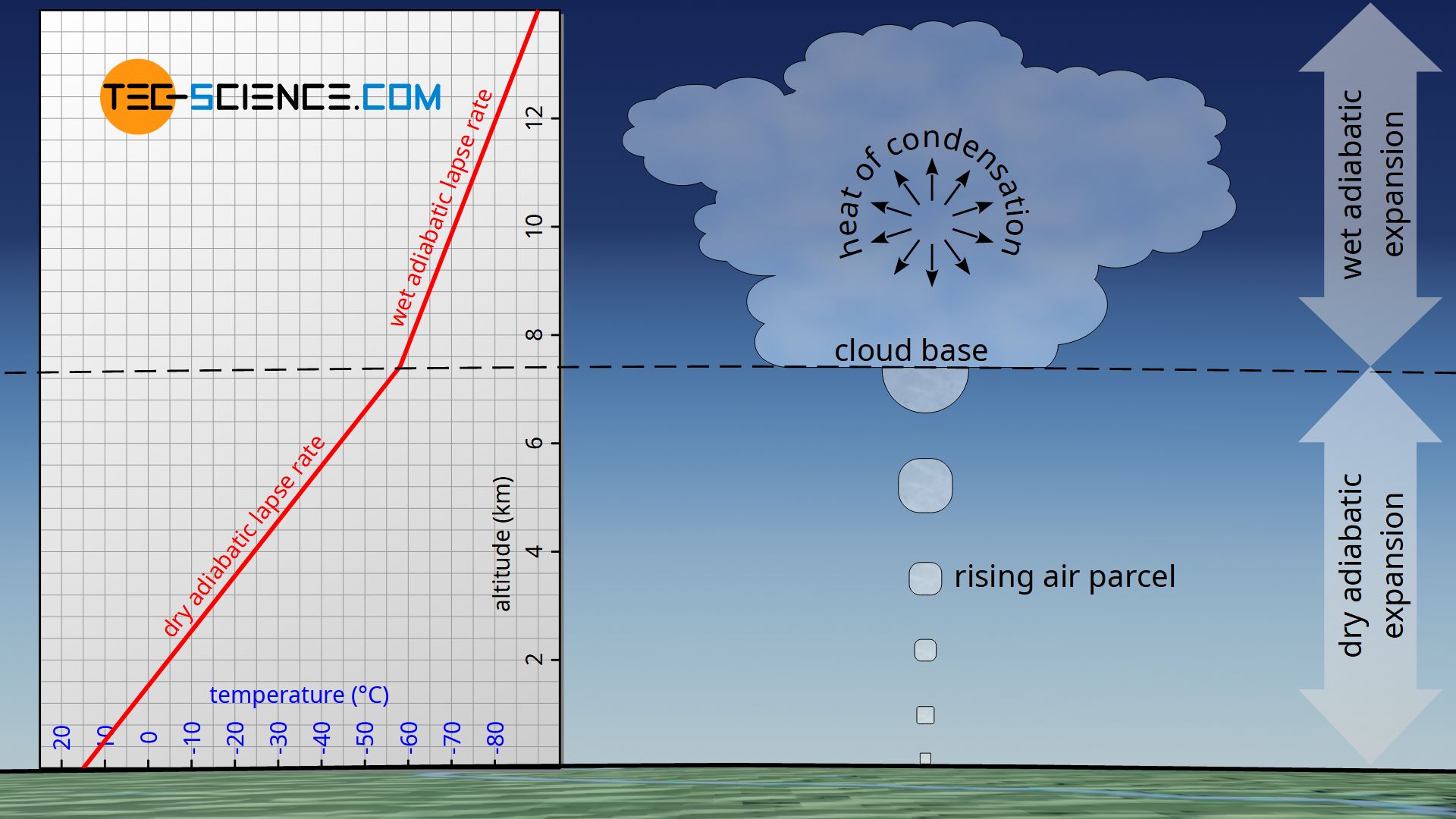
From a thermodynamic point of view, the formation of clouds is accompanied by an important phenomenon. The heat of condensation (also called latent heat) released during the condensation of water counteracts the cooling of the air. Thus, above the cloud base, an rising air parcel does not cool down as much as it does below the cloud base. Consequently, the lapse rate during condensation is lower than without cloud formation. Consequently, a distinction is made between the dry adiabatic lapse rate (without condensation) and the wet adiabatic lapse rate (with condensation).

In contrast to the dry adiabatic lapse rate, the wet adiabatic lapse rate takes into account the condensation of water vapor with increasing altitude! Due to the released heat of condensation, the wet adiabatic lapse rate is lower than the dry adiabatic one.

For the so-called standard atmosphere, the wet adiabatic lapse rate is assumed to be 0.65 °C/100m for the first 11 km above sea level. More about the standard atmosphere later in a separate section.

Pressure profile for an adiabatic atmosphere

Since now the temperature as a function of altitude is known according to the equation (\ref{th}), this function can be taken into account in deriving the pressure profile from the equation (\ref{c}).

\begin{align}
&\text{d}p = -\frac{g}{R_s \cdot T(h)} \cdot p \cdot \text{d} h \\[5px]
&\text{d}p = -\frac{g}{R_s \cdot \left(T_0 + \Gamma \cdot h \right)} \cdot p \cdot \text{d} h \\[5px]
&\frac{\text{d}p}{p} = -\frac{g}{R_s} \cdot \frac{\text{d} h}{ T_0 +\Gamma \cdot h } \\[5px]
\end{align}

Both sides of the equation can now be integrated within the corresponding limits. The lower limits refer to the reference level, i.e. h₀=0 and p₀. The upper limit corresponds to any altitude h at which the pressure p is to be determined.

\begin{align}
\label{p0}
&\boxed{\int_{p_0}^p~\frac{\text{d}p}{p} = -\frac{g}{R_s} \cdot \int_{h_0=0}^h\frac{\text{d} h}{T_0+\Gamma \cdot h}} \\[5px]
\end{align}

The left side of this equation yields the already known expression ln(p/p₀) [see derivation of equation (\ref{bar})]. For solving the integral on the right side of this equation a look into the formula collection of mathematics helps. For the case of a linear function in the denominator of a fraction the following indefinite integral results:

\begin{align}
&\int \frac{\text{d}x}{b+a \cdot x} = \frac{1}{a} \cdot \ln\left(b+a\cdot x\right) \\[5px]
\end{align}

This equation can now be applied to our case. With x=h, b=T₀ and a=Γ, the following solution results for the integral on the left side of equation (\ref{p0}):

\begin{align}
\int_{0}^h\frac{\text{d} h}{T_0 +\Gamma \cdot h} &= \left[\frac{1}{\Gamma} \cdot \ln\left(T_0+\Gamma \cdot h\right) \right]^h_0 \\[5px]
&= \frac{1}{\Gamma} \cdot \ln\left(T_0+\Gamma \cdot h\right) – \frac{1}{\Gamma} \cdot \ln\left(T_0\right) \\[5px]
&= \frac{1}{\Gamma} \cdot \left[ \ln\left(T_0+\Gamma \cdot h\right) -\ln\left(T_0\right)\right] \\[5px]
&= \frac{1}{\Gamma} \cdot \ln\left(\frac{T_0+\Gamma \cdot h}{T_0}\right) \\[5px]
& = \frac{1}{\Gamma} \cdot \ln\left(1+\frac{\Gamma}{T_0} \cdot h\right) \\[5px]
\end{align}

Equation (\ref{p0}) is thus represented as follows:

\begin{align}
\color{red}{\int_{p_0}^p~\frac{\text{d}p}{p}} &= -\frac{g}{R_s} \cdot \color{blue}{\int_{h_0=0}^h\frac{\text{d} h}{T_0 +\Gamma \cdot h}} \\[5px]
\color{red}{\ln\left(\frac{p}{p_0}\right) } &= -\frac{g}{R_s} \cdot \color{blue}{ \frac{1}{\Gamma} \cdot \ln\left(1+\frac{\Gamma}{T_0} \cdot h\right) } \\[5px]
\end{align}

This equation can be solved with respect to the pressure p by first applying the exponential function on both sides and then simplifying the resulting equation with the help of various logarithmic identities (e.g: e^ln(x)=x und \(\text{e}^{a \cdot b}= \left(\text{e}^{a}\right)^b\)):

\begin{align}
\text{e}^{\ln\left(\frac{p}{p_0}\right)} &= \text{e}^{-\frac{g}{R_s \cdot \Gamma} \cdot \ln\left(1+\frac{\Gamma}{T_0} \cdot h\right)}\\[5px]
\frac{p}{p_0} &= \left(\text{e}^{\ln\left(1+\frac{\Gamma}{T_0} \cdot h\right)} \right)^{ -\frac{g}{R_s \cdot \Gamma }}\\[5px]
\frac{p}{p_0} &= \left(1+\frac{\Gamma}{T_0} \cdot h\right)^{ -\frac{g}{R_s \cdot \Gamma }} \\[5px]
\end{align}

\begin{align}
\label{ext}
&\boxed{p(h) = p_0 \cdot \left(1+\frac{\Gamma}{T_0} \cdot h\right)^{ -\frac{g}{R_s \cdot \Gamma }}}~~~\text{barometric formula for an adiabatic atmosphere} \\[5px]
\end{align}

The equation above gives the pressure at any height h above a reference level, taking into account a linear temperature profile (adiabatic atmosphere). Note that the lapse rate Γ is to be used negatively in this equation. The lapse rate must be given in the unit K/m (“Kelvin per meter”) and the temperature T₀ in Kelvin.

The figure below shows the comparison of the classical barometric formula for an isothermal atmosphere with the extended barometric formula for an adiabatic atmosphere.

Density profile for an adiabatic atmosphere

Since, assuming an adiabatic system, the pressure is directly related to the volume and thus to the density. In this way the barometric formula can also be formulated for the density. For an adiabatic process, pressure and volume of two states are related to each other by the following equation:

\begin{align}
&p \cdot V^\gamma = p_0 \cdot V_0^\gamma \\[5px]
\end{align}

In this equation, pressure p₀ and volume V₀ refer to a considered air parcel at the reference level and p and V refer to the state at any height h. At constant mass – the mass of the air parcel does not change while rising – volume and density are in inverse relationship to each other (ϱ=m/V). Therefore, the following relationship applies between pressure and density:

\begin{align}
& p \cdot \frac{1}{\rho^\gamma} = p_0 \cdot \frac{1}{\rho_0^\gamma} \\[5px]
& \frac{p}{\rho^\gamma} = \frac{p_0}{\rho_0^\gamma} \\[5px]
& p = p_0 \cdot \left(\frac{\rho}{\rho_0}\right)^\gamma \\[5px]
\end{align}

This formula for the pressure is now used in equation (\ref{ext}) and solved with respects to the density ϱ:

\begin{align}
\require{cancel}
p &= p_0 \cdot \left(1+\frac{\Gamma}{T_0} \cdot h\right)^{ -\frac{g}{R_s \cdot \Gamma }} \\[5px]
\bcancel{p_0} \cdot \left(\frac{\rho}{\rho_0}\right)^\gamma &= \bcancel{p_0} \cdot \left(1+\frac{\Gamma}{T_0} \cdot h\right)^{ -\frac{g}{R_s \cdot \Gamma }} \\[5px]
\frac{\rho}{\rho_0} &= \left(1+\frac{\Gamma}{T_0} \cdot h\right)^{ -\frac{g}{\gamma \cdot R_s \cdot \Gamma }} \\[5px]
\end{align}

\begin{align}
\boxed{\rho(h) = \rho_0 \cdot \left(1+\frac{\Gamma}{T_0} \cdot h\right)^{ -\frac{g}{\gamma \cdot R_s \cdot \Gamma }}} \\[5px]
\end{align}

Formally, the formula for the density differs from the formula for the pressure only by the exponent, which at this point is divided by the heat capacity ratio.

The standard atmosphere

The barometric formula for an adiabatic atmosphere is used to describe the so-called standard atmosphere up to an altitude of about 85 km. The atmosphere is divided into different layers, whereby a constant lapse rate is assumed within each layer.

Sea level (km)	Lapse rate (K/km)	Temperature (°C)
0	-6,5	15,0
11	+0,0	-56,5
20	+1,0	-56,5
32	+2,8	-44,5
47	+0,0	-2,5
51	-2,8	-2,5
71	-2,0	-58,5
85		-84,3

Source: https://ntrs.nasa.gov/archive/nasa/casi.ntrs.nasa.gov/19770009539.pdf

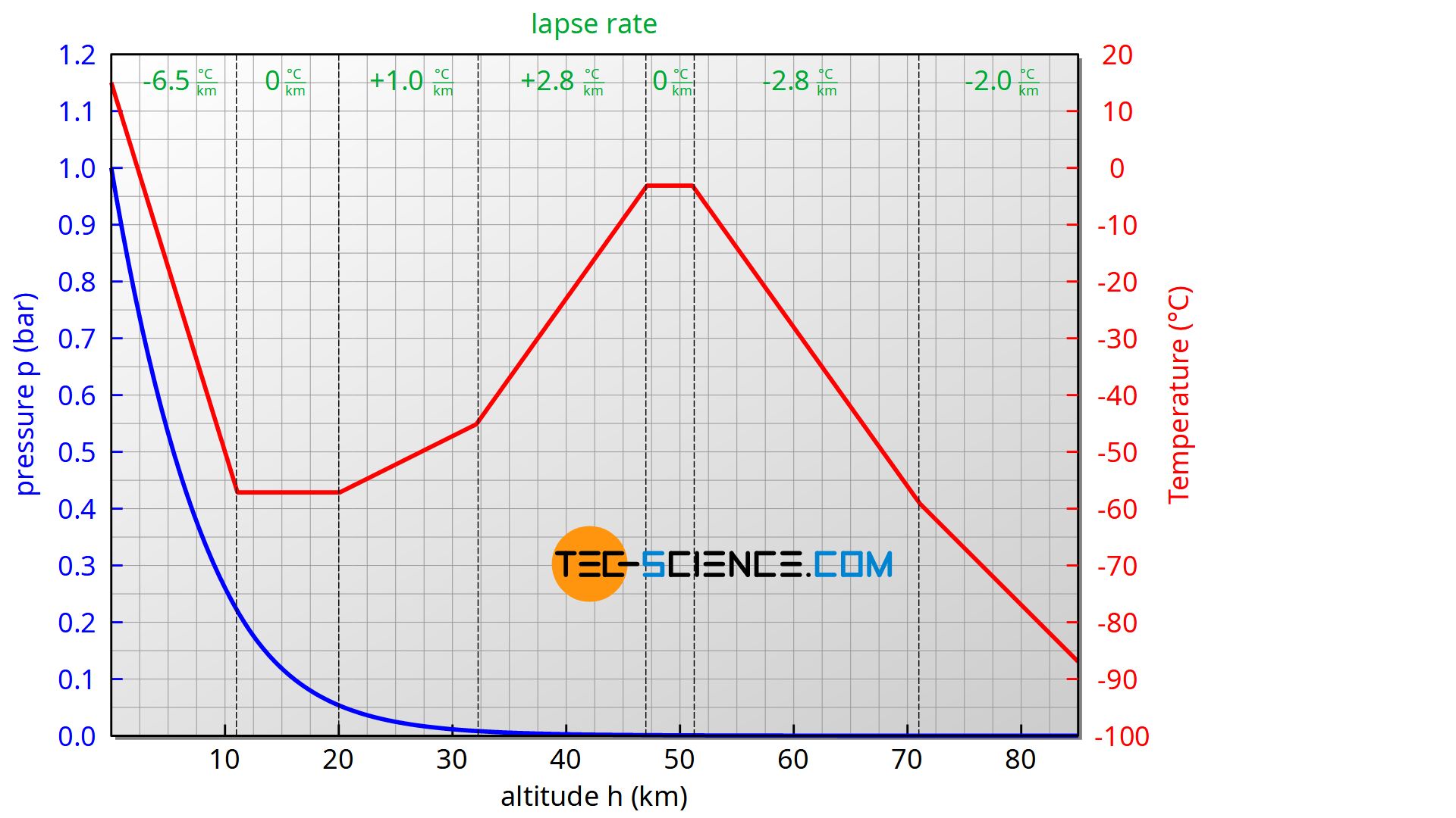
The increase in temperature in the stratosphere (from about 20 km) is mainly due to the absorption of UV radiation by the ozone layer. The temperature then drops again to a minimum of around -86 °C at about 90 km. From 100 km the temperature rises rapidly again and even exceeds 700 °C at 300 km! The reason for this is the low air density and the associated large mean free path. This allows the molecules to travel long distances without collisions. This leads to relatively high molecular speeds and thus to high temperatures. Due to the fact that there are only a few molecules, the associated internal energy of the gas is therefore very low despite the high temperature. Therefore one would freeze to death despite the high temperatures, because only very little heat is transferred!

Note that when describing the pressure in an isothermal layer, the barometric formula for an adiabatic atmosphere cannot be used. The lapse rate in this case is zero, but it is the denominator of the fraction in the exponent. There is no mathematical solution for this. In this case, either a sufficiently small lapse rate must be assumed so that the error made is kept to a minimum, or the “classical” barometric formula for an isothermal atmosphere must be used.