At a certain optimum belt speed, a belt drive can transmit the maximum possible power.
Introduction
In the article Mechanical power it was shown that an object that is moved by a force F with the speed v converts the power P=F⋅v. Applied to the belt drive, this means that if the belt is moved by the circumferential force Fc at the speed v, the belt transmits the following power:
\begin{align}
\label{leistung}
\boxed{P=F_c \cdot v} \\[5px]
\end{align}
This power is transmitted from the drive pulley to the belt and then to the output pulley. Note that a belt drive (and a transmission in general) does not change the power! The belt merely serves as a “transmitter” oft the power between the input and the output pulley, so to speak. However, due to its limited strength, the belt cannot transmit any high power and it can even achieve an optimum belt speed at which the maximum power is reached, as will be explained in more detail in the following sections.
Influence of circumferential force and belt speed on the transmitted power
First of all, according to the equation (\ref{leistung}), a high power to be transmitted also means a high speed. However, high speeds lead to an increase in centrifugal forces. Since the allowable belt stress in the belt is limited, the increase in centrifugal forces is at the expense of the maximum permissible tight side force. This is also directly illustrated by the equation derived in the article Maximum belt stress, in which the sum of tight side stress σt, bending stress σb and speed-dependent centrifugal stress σcf(v) must not exceed the maximum permissible overall stress σper:
\begin{align}
&\sigma_t + \sigma_b + \sigma_{cf}(v) \le \sigma_{per} \\[5px]
\label{zulaessige}
&\boxed{\sigma_{t,per} \le \sigma_{per} -\sigma_b – \sigma_{cf}(v)} ~~~\text{and}~~~\boxed{\sigma_{cf}(v) = \rho \cdot v^2} ~~~\text{and}~~~ \boxed{\sigma_b =E_b \cdot \frac{s}{d + s}}\\[5px]
\end{align}
The permissible tensile stress σt,per decreases with increasing centrifugal stress σcf(v). This is then directly connected with a decrease of the maximum transferable circumferential force Fc,max. Because at a given tight side force (which in this case corresponds to the maximum permissible force Ft,per= σt,per⋅A), only a certain circumferential force Fc,max can be transmitted. The connection between the circumferential force and the tight side force is established by the so-called “gain” k and only dependent on the wrap angle φ and the friction coefficient µ:
\begin{align}
&F_{c,max} = F_{t,per} \cdot k \\[5px]
\label{nutzkraft}
&\boxed{F_{c,max} = \sigma_{t,per} \cdot A \cdot k} ~~~\text{and}~~~ \boxed{k= \left(1- \frac{1}{e^{\mu \cdot \varphi}} \right) } ~~~\text{“yield”} \\[5px]
\end{align}
According to the equation (\ref{leistung}), low circumferential forces in turn lead to a decrease in power. In extreme cases of high speeds, the centrifugal forces are so high that no circumferential force can be transmitted at all (and thus no power), as otherwise the allowable belt stress would immediately be exceeded. Excessively high belt speeds therefore prohibit the transmission of high power!
Increasing belt speeds lead to a decrease in the transmissible circumferential force, as the centrifugal force would otherwise place an unacceptably high load on the belt! The transmitted power decreases!
Conversely, at low speeds, larger circumferential forces and thus superficially higher performances can be achieved; however, if this results in the belt speed having to be reduced to such an extent (otherwise the centrifugal forces would become too high) that the belt hardly moves any more, then there is no great power behind the large circumferential force anyway!
Decreasing belt speeds lead to an increase in the transmissible circumferential force, but the transmitted power decreases!
In fact, belt drives have an economically optimal belt speed at which the maximum power Pmax can be transmitted, i.e. an optimal force/speed ratio is available. This optimum belt speed will be discussed in more detail in the next section.
Optimum belt speed
Maximum transmittable power
To determine the optimum belt speed vopt, the equations (\ref{zulaessige}), (\ref{nutzkraft}) and (\ref{leistung}) must be combined to first express the maximum transmissible power Pmax as a function of the belt speed v:
\begin{align}
&P_{max} = F_{c,max} \cdot v \\[5px]
&P_{max} = \sigma_{t,per} \cdot A \cdot k \cdot v \\[5px]
&P_{max} = \left( \sigma_{per} -\sigma_b – \sigma_{cf}(v) \right) \cdot A \cdot k \cdot v \\[5px]
&P_{max} = \left( \sigma_{per} – \sigma_b – \rho \cdot v^2 \right) \cdot A \cdot k \cdot v \\[5px]
\end{align}
If the cross-sectional area A of the flat belt is expressed by its belt thickness s and its belt width b (A=b⋅s), then the maximum transmissible power Pmax at a given speed v finally results as follows:
\begin{align}
\label{abs_leistung}
&\boxed{P_{max}(v) = \left( \sigma_{per} – \sigma_b – \rho \cdot v^2 \right) \cdot b \cdot s \cdot k \cdot v} \\[5px]
\end{align}
Note that for the gain k the smallest wrap angle of the two pulleys is decisive! In general this applies to the smaller pulley, especially as the greatest bending stresses also act there. Both the wrap angle φ (relevant for the gain) and the pulley diameter d (relevant for the bending stress) therefore refer to the smallest of the pulleys.
Specific power (“power per unit belt width”)
Often the power Pmax is related to the belt width b and is then called specific power pmax (“power per unit belt width”). This makes sense because the belt thickness s for calculating the bending stress σb must be assumed in advance anyway. This leaves the belt width as the only unknown geometric parameter b. It therefore makes sense to first express the power independently of the belt width and to state it as specific power:
\begin{align}
&p_{max} = \frac{P_{max}}{b} \\[5px]
\label{spez_leistung}
&\boxed{p_{max} (v) =\left( \sigma_{per} – \sigma_b – \rho \cdot v^2 \right) \cdot s \cdot k \cdot v} \\[5px]
\end{align}
The specific power is the power per unit belt width!
Based on this maximum transmittable specific power pmax, the required belt width breq to transmit the nominal power Pn is then determined in practice. For safety reasons, various operating factors C are taken into account, which include the influence of impulsive torque loads and various environmental influences which could lead to friction reduction:
\begin{align}
&\boxed{b_{req} =\frac{P_n}{p_{max} \cdot C} } \\[5px]
\end{align}
Maximum power as a function of speed
The figure below shows the maximum transmittable specific power pmax as a function of the belt speed v according to the equation (\ref{spez_leistung}) for the values given in the diagram. It is now also graphically clear that neither too low nor too high belt speeds lead to an arbitrarily high transmittable power. There is a pronounced maximum in which the greatest possible maximum power can be transmitted.
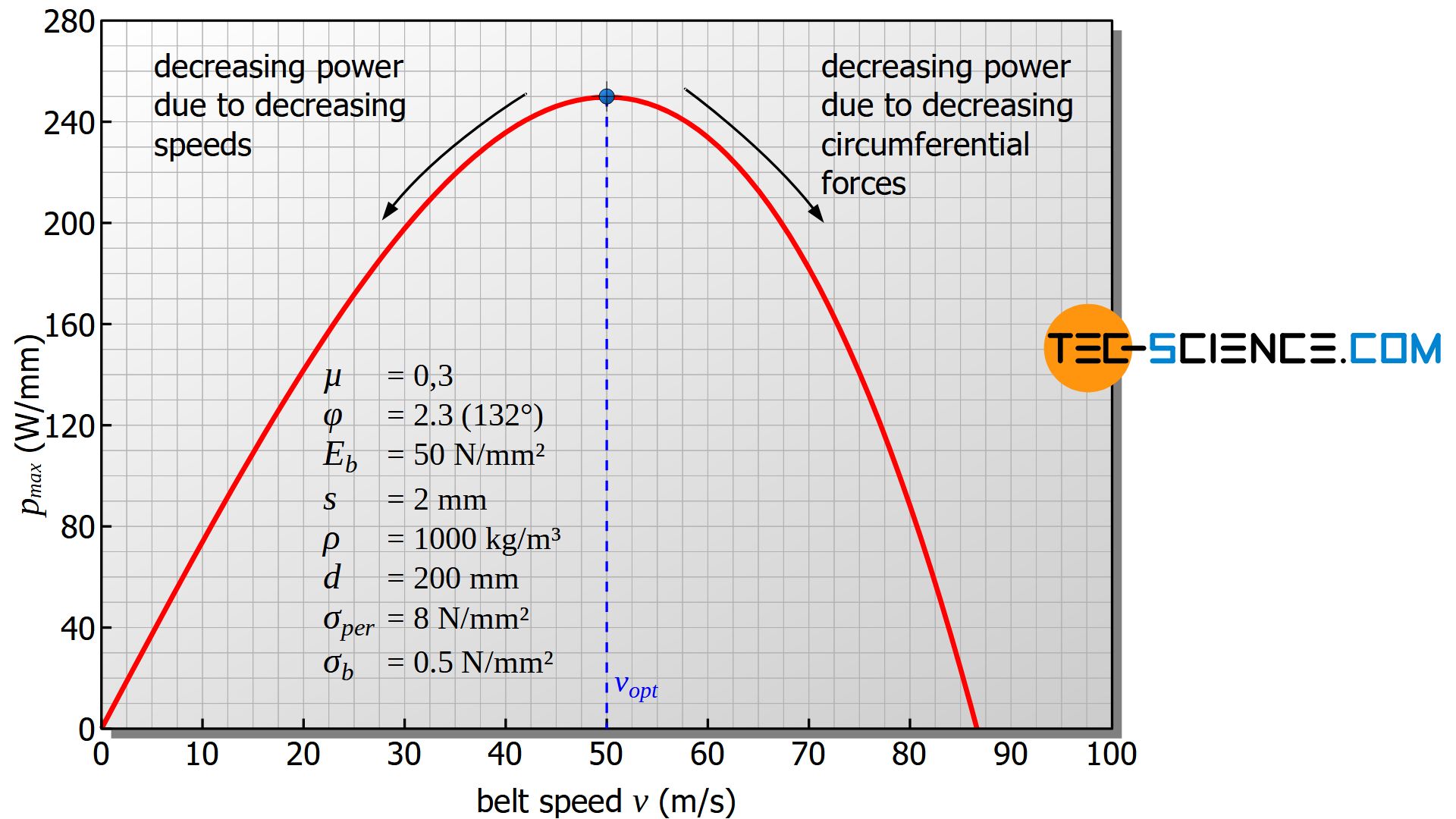
To reach this maximum, the belt speed must be set to the optimum. This is also called optimum belt speed and in the present case is about 50 m/s and corresponds to a rotational speed of the smaller pulley of 4774 min-1. As this example shows, the optimum belt speeds are often very high and are usually not achieved in practice.
There is an optimal belt speed at which the maximum power can be transmitted!
Calculation of the optimum belt speed
To calculate the optimum belt speed, the maximum value of the function pmax(v) or Pmax(v) must be found. Mathematically, this corresponds to zeroing the first derivative:
\begin{align}
&\frac{\text{d}p_{max}(v)}{\text{d}v} = 0 \\[5px]
&\left( \sigma_{per} – \sigma_b – 3 \rho \cdot v^2 \right) \cdot s \cdot k = 0 \\[5px]
&\sigma_{per} – \sigma_b – 3 \rho \cdot v^2 = 0 \\[5px]
\label{v_opt}
&\boxed{v_{opt} = \sqrt{\frac{\sigma_{per} – \sigma_b }{3 \rho}}} ~~~\text{and}~~~ \boxed{\sigma_b = E_b \cdot \frac{s}{d + s}}\\[5px]
\end{align}
At the given transmission ratio and speed of the drive pulley, the belt speed can be adjusted by larger or smaller pulleys in order to achieve the optimum belt speed. However, in order not to change the desired transmission ratio, both pulleys (driving and driven pulley) must always be changed to the same extent. Note that changing the pulley diameter changes the bending stress and thus the optimum belt speed!
The maximum specific power pmax,opt or absolute power Pmax,opt, which can be transmitted at the optimum belt speed vopt, is then obtained by applying equation (\ref{v_opt}) to equation (\ref{spez_leistung}) or (\ref{abs_leistung}):
\begin{align}
&\boxed{p_{max, opt} = k \cdot \sqrt{\frac{4 \left(\sigma_{per} – \sigma_b \right)^3 }{27 \rho}}} \\[5px]
&\boxed{P_{max, opt} = k \cdot b \cdot \sqrt{\frac{4 \left(\sigma_{per} – \sigma_b \right)^3 }{27 \rho}}} \\[5px]
\end{align}


