The Hagen-Poiseuille equation for describing the parabolic velocity profile of fluids in pipes applies only to long pipes for energy reasons!
Summary
As derived in detail in the article on the Hagen-Poiseuille equation, the Poiseuille flow with its typical parabolic velocity profile can be described by the following equations:
\begin{align}
\label{vrr}
&\boxed{v(r)=v_\text{max} \cdot \left[1-\left(\frac{r}{R}\right)^2\right]} \\[5px]
\label{max}
&\boxed{v_{\text{max}}= -\frac{R^2}{4\eta} \frac{\text{d} p}{\text{d}x} } \\[5px]
\label{pv}
& \boxed{\frac{\text{d}p}{\text{d}x} = \frac{\Delta p}{ \Delta L}} \\[5px]
\label{loss}
& \boxed{\Delta p_l = \frac{8\eta \cdot \Delta L}{R^2} \cdot c} ~~~\text{pressure loss} \\[5px]
\label{vmax}
& \boxed{c = \frac{1}{2} \cdot v_\text{max}} \\[5px]
\end{align}

In these equations, ΔL denotes the length of the pipe section and R is the inner radius of the pipe. v(r) denotes the velocity of the fluid at a distance r from the pipe axis and η is the viscosity of the fluid. The pressure gradient dp/dx is the drive for the flow and corresponds to the pressure change per unit length. The pressure gradient is determined by the pressure change Δp along the pipe. The mean flow velocity c corresponds to just half of the maximum flow velocity vmax in the middle of the pipe.
Startup (formation of the laminar flow profile)
The pressure gradient dp/dx in the above equation is required to compensate for friction losses, so that the fluid keeps flowing. However, a flow is not “just there”, it must be created. In other words, the fluid must first be accelerated to the characteristic parabolic flow profile. The relationships derived and explained in the article on the Hagen-Poiseuille equation therefore only apply to pipe sections in which the flow profile has already been fully developed. So also the above equations.
In the following we would therefore like to go into the entire flow process in more detail. For this purpose we imagine a large tank that is completely filled with a liquid. At the bottom of the tank, a horizontal pipe is connected to the side, through which the fluid flows into the open. The tank is so large that the liquid level does not sink noticeably when the fluid flows out. The liquid does not move inside the tank, so to speak, but is obviously accelerated through the pipe into the open.
The distance that the fluid travels in the pipe until the parabolic flow profile has fully developed is referred to as the inlet length or startup length. The flow along the startup length is called the inlet flow or startup flow. The figure below shows the velocity distribution at various points in the pipe.
The flow can be divided into three parts:
- acceleration to the constant inlet velocity and
- subsequent acceleration to the parabolic velocity profile,
- as well as the friction that has to be permanently compensated.
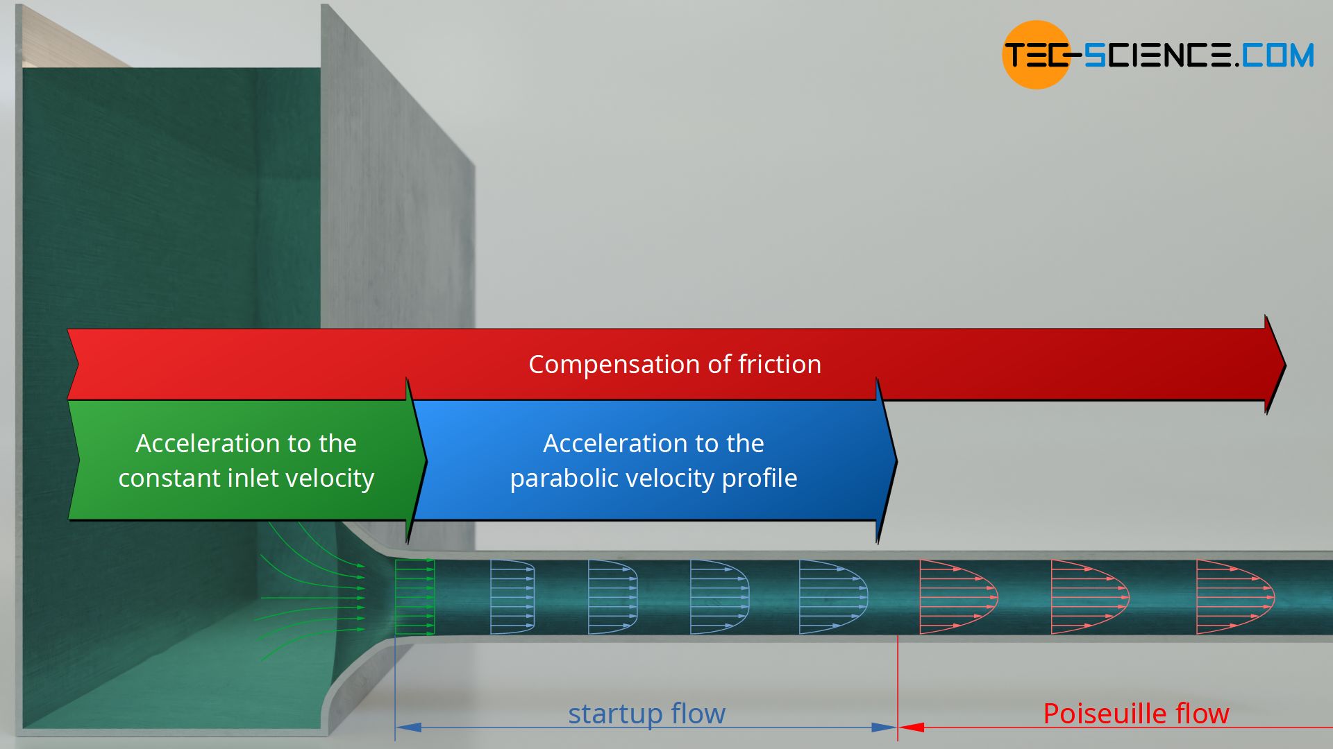
All three processes are associated with a corresponding energy input and thus with a pressure drop. This will be discussed in more detail below.
Acceleration to the constant inlet velocity (inlet flow)
The fluid is first accelerated in the tank at the level of the pipe axis up to the beginning at the inlet (intake flow). It enters the streamlined, rounded inlet at an almost constant speed c. The rounding is decisive in practice, since otherwise the flow profile would be narrowed at sharp-edged transitions due to the so-called vena contracta, which would result in a reduction of the flow rate (for further information see article Discharge of liquids).
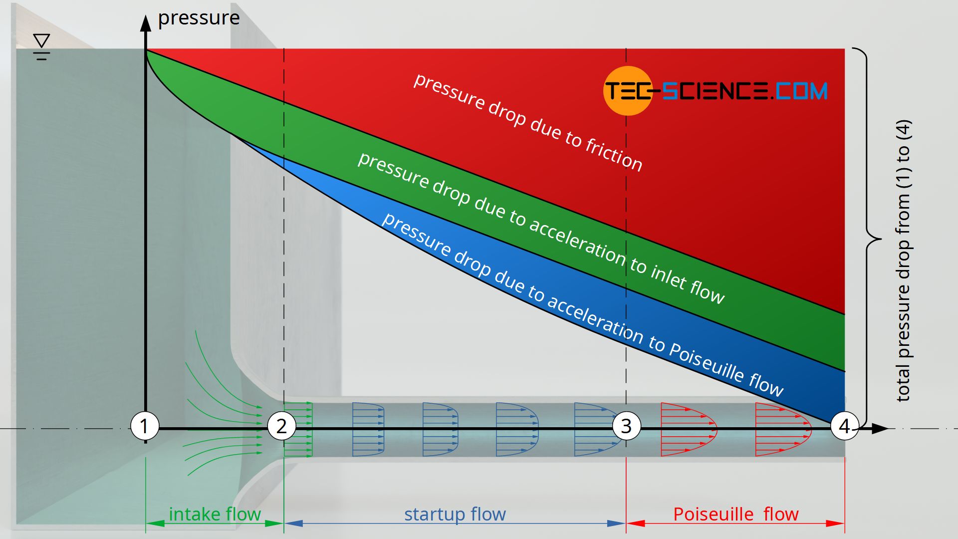
If the pressure p1 acts in the resting fluid at the level of the pipe axis, part of this pressure is thus used for accelerating the liquid to the constant inlet velocity c. According to Bernoulli’s equation, this leads to a reduction of the (static) pressure at the inlet to a value p2. This pressure drop Δpa1 due to the acceleration of the liquid is determined as follows:
\begin{align}
&p_2 = p_1 – \frac{\rho}{2} c^2 \\[5px]
\label{p}
&\Delta p_{a1} =p_1-p_2= \frac{\rho}{2} c^2 \\[5px]
\end{align}
Acceleration to the parabolic velocity profile (Poiseuille flow)
After the fluid has been accelerated up to the inlet to the constant inlet speed c, the friction between the fluid and the pipe wall begins to take effect over the startup length (this transition from intake flow to startup flow is smooth). The fluid there adheres to the wall, so that the flow velocity at the wall is zero (no-slip condition). Due to the viscosity, the fluid layers further away from the wall are decelerated more and more.
Despite the velocity reduction near the pipe wall, the same mass must still flow through the pipe due to the conservation of mass (continuity equation). So while the flow velocity decreases towards the wall, the velocity at the center region of the pipe (core flow) must increase compared to the inlet velocity. Often the core flow along the startup length is regarded as an area with constant velocity. Towards the edge, the speed then decreases parabolically to zero. At a certain distance, a continuous parabolic profile has finally developed. This marks the end of the startup length.
One could be jumping to the conclusion that the formation of the parabolic velocity profile does not require any additional energy, because after all, the fluid loses velocity near the wall of the pipe to the same extent as it gains velocity near the center of the pipe. This may be true for velocity, but not for kinetic energy. The kinetic energy is related quadratically to the speed. In addition, the velocity profile itself is parabolic, so that the higher velocity components in the middle of the flow have much more influence on the kinetic energy.
The loss of kinetic energy near the wall does not outweigh the kinetic energy required to accelerate the fluid near the center. Additional energy is therefore required to form the parabolic velocity profile out of the the constant inlet velocity profile! This additional energy corresponds to the amount of kinetic energy of the startup flow. Analogous to the equation (\ref{p}), a further pressure drop Δpa2 occurs due to the energy required to form the parabolic flow profile. In fact, this required energy is identical with equation (\ref{p}) (will be shown in the last section of this article):
\begin{align}
\label{pp}
&\Delta p_{a2} = \frac{\rho}{2} c^2 \\[5px]
\end{align}
In total, therefore, the following pressure drop occurs during the acceleration process of the fluid:
\begin{align}
&\Delta p_{a} =\Delta p_{a1} + \Delta p_{a1} \\[5px]
\label{ppp}
&\boxed{\Delta p_{a} = \rho c^2} ~~~~~\text{correction term} \\[5px]
\end{align}
For the total pressure drop, the actual friction losses according to equation (\ref{loss}) must of course be taken into account (note that this term is also present along the startup length, because regardless of whether the flow profile has formed or not, frictional forces described by this term act):
\begin{align}
&\Delta p = \Delta p_a + \Delta p_V \\[5px]
&\boxed{\Delta p = \frac{8\eta \cdot L}{R^2} \cdot c + \rho c^2} \\[5px]
\end{align}
Discussion
From this equation it can be seen that, in the case of a pressure drop along a pipe, the kinetic energies for accelerating the fluid must usually also be taken into account. But this equation also shows, that for long pipe lengths L with at the same time small radii R, the term used to describe the frictional losses becomes larger than the term used to describe the acceleration.
In fact, Poiseuille initially failed to recognise the need to take into account the pressure losses due to the acceleration. The result was incorrect predictions of the volume flow rate, especially with short pipes. Only when Hagen corrected his equations by the term (\ref{ppp}) did the theoretical predictions agree with practice. This acceleration term is therefore also called the correction term.
If, by the way, the pipe would not be arranged horizontally, but would overcome a height Δh, then potential energy would have to be added to the fluid. This would lead to a further pressure drop Δph=ϱ⋅g⋅Δh! More on this topic in the article Bernoulli’s principle.
Minimum ratio of pipe length to pipe diameter
Acceleration energy (microscopic analysis of the flow)
In the following, the Poiseuille flow will be examined more closely from an energetic point of view. In a pipe section of the length ΔL the kinetic energy of the flow is to be determined on a microscopic level. For this purpose we consider a hollow cylinder with a radius r and a thickness dr. The height of this cylinder corresponds to the length ΔL of the pipe section. The fluid mass contained in this hollow cylinder is determined by the following formula:
\begin{align}
\label{dm}
&\text{d}m = \overbrace{\underbrace{2\pi r \cdot \text{d}r}_{\text{d}A} \cdot \Delta L}^{\text{d}V}\cdot \rho \\[5px]
\end{align}
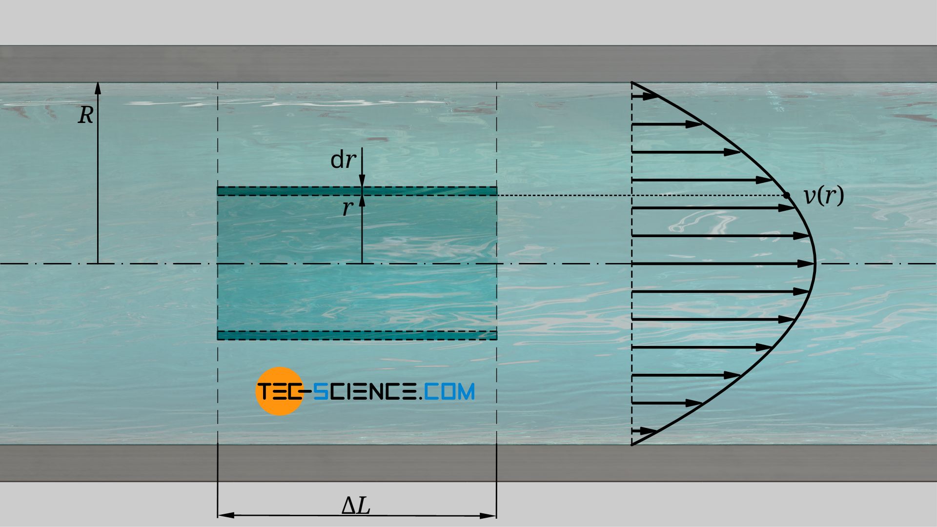
The velocity of this mass at the distance r is given by equation (\ref{vrr}), so that for the kinetic energy dWkin applies:
\begin{align}
\text{d}W_\text{kin} &= \frac{1}{2} \text{d}m \cdot v^2(r) \\[5px]
&= \frac{1}{2} \overbrace{2\pi r \cdot \text{d}r \cdot \Delta L \cdot \rho}^{\text{d}m} \cdot v^2(r) \\[5px]
&= \pi r \rho \Delta L \cdot v^2(r) \cdot \text{d}r \\[5px]
&= \pi r \rho \Delta L \cdot v_\text{max}^2 \cdot \left[1-\left(\frac{r}{R}\right)^2\right]^2 \cdot \text{d}r \\[5px]
&= \pi \rho \Delta L \cdot v_\text{max}^2 \cdot \left(r-\frac{2r^3}{R^2} +\frac{r^5}{R^4} \right) \cdot \text{d}r \\[5px]
\end{align}
The kinetic energy Wkin inside the entire pipe section is finally obtained by integrating this equation within the limits from r=0 to r=R:
\begin{align}
W_\text{kin} &= \int \text{d} P_\text{kin} = \pi\rho \Delta L ~v_\text{max}^2 \cdot \int \limits_0^R \left(r-\frac{2r^3}{R^2} +\frac{r^5}{R^4} \right) \cdot \text{d}r \\[5px]
&= \pi\rho\Delta L~v_\text{max}^2 \cdot \left\vert \frac{r^2}{2}-\frac{r^4}{2R^2} +\frac{r^6}{6R^4}\right\vert_0^R \\[5px]
&= \pi\rho \Delta L~ v_\text{max}^2 \cdot \left( \frac{R^2}{2}-\frac{R^4}{2R^2} +\frac{R^6}{6R^4} \right) \\[5px]
&= \pi\rho \Delta L~ v_\text{max}^2 \cdot \frac{R^2}{6} \\[5px]
\end{align}
By rearranging this equation, the kinetic energy can also be expressed as a function of the mean flow velocity c:
\begin{align}
W_\text{kin} &= \pi\rho \Delta L~ v_\text{max}^2 \cdot \frac{R^2}{6} \\[5px]
&= \pi\rho \Delta L~ v_\text{max} \cdot \underbrace{\frac{v_\text{max}}{2}}_{c} \cdot \frac{R^2}{3} \\[5px]
&= \pi\rho c \Delta L~ v_\text{max} \cdot \frac{R^2}{3} \\[5px]
\end{align}
If the relationship according to the equation (\ref{max}) is used for the maximum flow velocity, then the kinetic energy can be determined on the basis of the pressure gradient (at this point only the magnitude of the pressure gradient should be considered, without sign):
\begin{align}
W_\text{kin} &= \pi\rho c \Delta L \cdot \overbrace{\frac{R^2}{4\eta} \frac{\text{d} p}{\text{d}x}}^{v_\text{max}} \cdot \frac{R^2}{3} \\[5px]
W_\text{kin} &=\frac{ \pi\rho c \Delta L R^4}{12\eta} \frac{\text{d} p}{\text{d}x} \\[5px]
\end{align}
For a pipe section of length ΔL and pressure drop Δp, the pressure gradient is given according to equation (\ref{pv}), so that the kinetic energy is determined from the pressure difference as follows:
\begin{align}
&W_\text{kin} =\frac{ \pi\rho c \Delta L R^4}{12\eta} \frac{\Delta p}{\Delta L} \\[5px]
\label{x}
&\boxed{W_\text{kin} =\frac{\pi\rho c R^4 \Delta p}{12 \eta}} \\[5px]
\end{align}
That kinetic energy of the flow corresponds to the work required for acceleration of the fluid.
Displacement energy (macroscopic analysis of the flow)
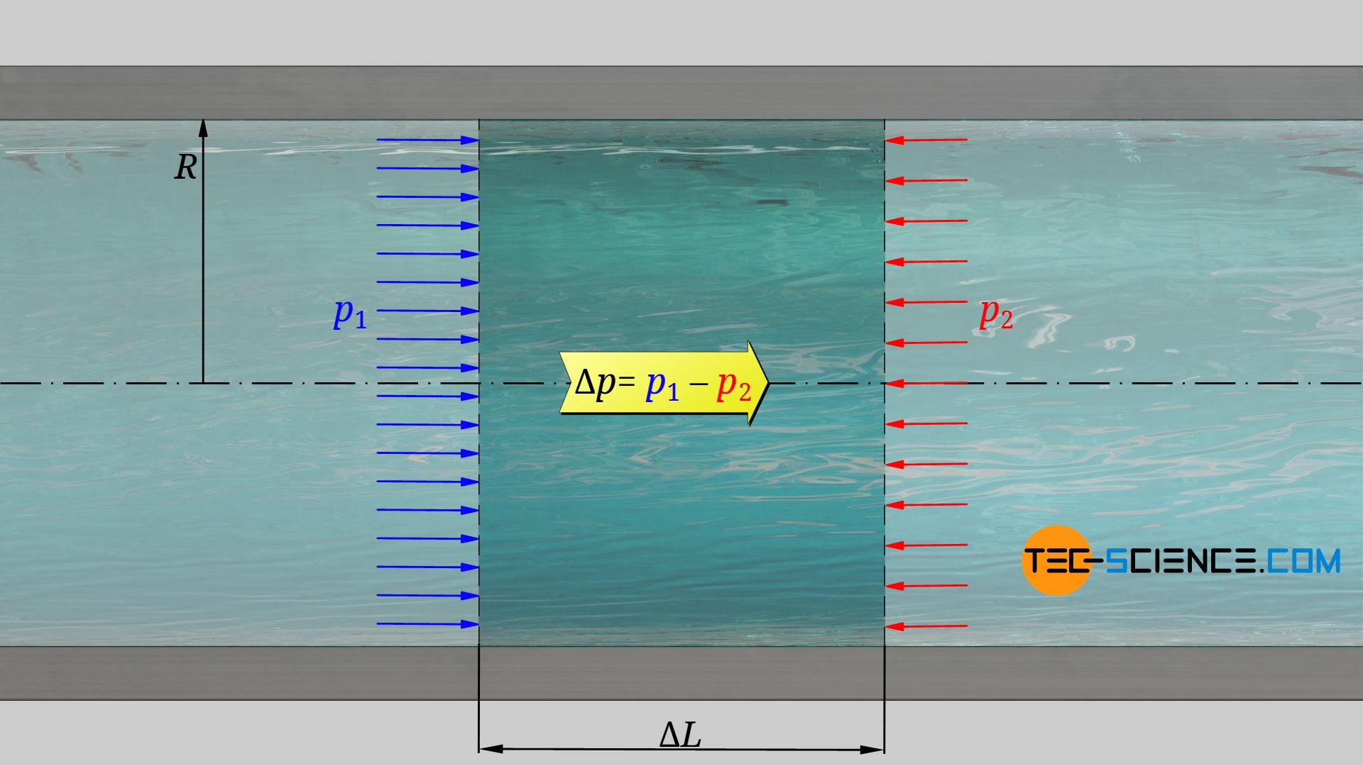
The flow of the fluid is caused by the fact that the fluid is pressed through the pipe due to a pressure difference. To displace the fluid through the pipe section, a certain force and thus energy. In order to determine this displacement energy, we no longer look at the fluid on a microscopic level, but on a macroscopic level.
The force required for displacing the fluid results from the difference in pressure between the start and end of the pipe and the cross-sectional area of the pipe:
\begin{align}
F = \Delta p \cdot A = \Delta p \cdot \pi R^2 \\[5px]
\end{align}
The energy applied when the fluid flows over the entire pipe section ΔL can thus be determined as follows:
\begin{align}
&W_V = F \cdot \Delta L \\[5px]
\label{y}
&\boxed{W_V = \Delta p \cdot \pi R^2 \Delta L} ~~~~~\text{displacement energy applied}\\[5px]
\end{align}
Minimum ratio of pipe length and pipe diameter
One can now estimate the minimum ratio between pipe length and pipe diameter for the validity of the Hagen-Poiseuille equation by the following consideration. The applied displacement energy is used to accelerate the fluid on the one hand and to overcome friction on the other hand. Since friction is always present, the energy required for acceleration according to equation (\ref{x}) cannot be greater than the applied displacement energy according to equation (\ref{y}). Therefore, the following condition must be fulfilled:
\begin{align}
\require{cancel}
W_V & >W_{\text{kin}} \\[5px]
\cancel{\Delta p} \cdot \cancel{\pi} R^2 \Delta L & > \frac{\cancel{\pi} \rho c R^4 \cancel{\Delta p}}{12 \eta}\\[5px]
\Delta L & > \frac{ \rho c R^2 }{12 \eta}\\[5px]
\Delta L & > \frac{ \rho c ~2R }{\eta}\cdot \frac{2R}{48}\\[5px]
\Delta L & > \color{red}{\frac{ \rho ~c ~D }{\eta}}\cdot \frac{D}{48}\\[5px]
\end{align}
The term marked in red (consisting of density, flow velocity, pipe diameter and viscosity) corresponds to the so-called Reynolds number. The minimum required ratio of pipe length to pipe diameter is therefore dependent on the Reynolds number:
\begin{align}
& \Delta L > \color{red}{Re}\cdot \frac{D}{48}\\[5px]
&\boxed{\frac{\Delta L}{D} > \frac{Re}{48}} \\[5px]
\end{align}
The ratio of length to radius of a pipe should be greater than one forty-eighth of the Reynolds number for the Hagen-Poiseuille law to be valid!
This statement must be further limited with regard to turbulent flows. There the Hagen-Poiseuille equation does not apply in principle. Practice shows that turbulent flows in pipes are to be expected from Reynolds numbers greater than 2300. In such a limiting case the length-diameter-ratio is about 50, i.e. the pipe would have to be about 50 times as long as its diameter for a parabolic velocity profile according to the Hagen-Poiseuille equation to be established.
Kinetic power of the constant startup flow compared to the parabolic velocity profile
In this section we will prove that the formation of the parabolic velocity profile requires the same energy as the formation of the constant startup flow from which it results. For this purpose we calculate the kinetic power with which the fluid flows through the cross-section of the pipe (kinetic energy per time unit).
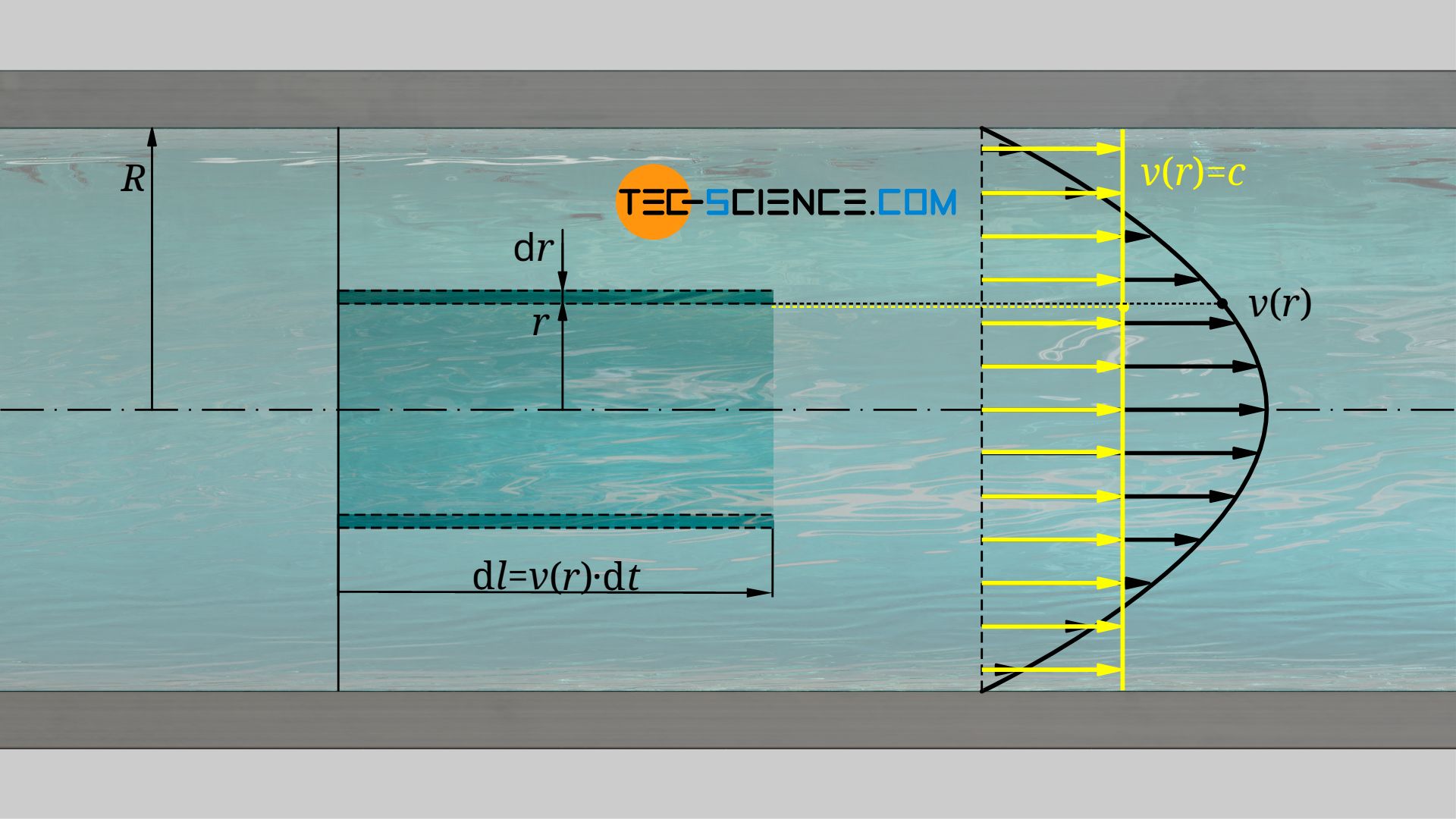
We consider a ring with a radius r from the center of the pipe and with the thickness dr. Within the time dt the fluid flows with the velocity v(r) through the surface dA=2π⋅r⋅dr. The fluid covers the distance dl=v(r)⋅dt. Thus, for the mass dm flowing through the ring surface, the following formula applies:
\begin{align}
& \text{d}m = \text{d}V \cdot \rho = \text{d}A\cdot \text{d}l \cdot \rho=2\pi r\cdot\text{d}r \cdot v(r)\cdot \text{d}t \cdot \rho\\[5px]
\end{align}
So within the time dt the below given amount of energy dWkin flows through the ring surface, from which the power can be calculated as energy per time unit dPkin:
\begin{align}
& W_\text{kin}= \frac{1}{2} \text{d}m~ v^2(r)= \pi\rho r\cdot v^3(r)\cdot \text{d}r ~\text{d}t \\[5px]
& \text{d}P_\text{kin}=\frac{W_\text{kin}}{\text{d}t} = \pi\rho r\cdot v^3(r)\cdot \text{d}r\\[5px]
\end{align}
The kinetic power through the entire pipe cross section is finally obtained by integrating this equation within the limits between r=0 and r=R:
\begin{align}
& \underline{P_\text{kin}=\pi\rho ~\int\limits_0^R r\cdot v^3(r)\cdot \text{d}r}\\[5px]
\end{align}
At the inlet of the pipe, the speed is constant over the entire cross-section (no function of radius). Due to the conservation of mass, this velocity corresponds to the mean flow velocity c of the Poiseuille flow. Thus, for a velocity profile with v(r)=c, that is constant over the entire cross-section, the following formula applies to the kinetic power:
\begin{align}
& P_\text{kin,1}=\pi\rho~c^3~\int\limits_0^R r \cdot \text{d}r =\pi\rho~\left\vert \frac{1}{2}r^2 \right\vert_0^R \\[5px]
& \boxed{P_\text{kin,1}=\frac{1}{2}\pi\rho~R^2~c^3} \\[5px]
\end{align}
This kinetic power corresponds to the power directly measured at the start of the startup length. Now we determine the kinetic power with the parabolic flow profile, i.e. the power after the startup length. In this case the velocity is a function of the radius according to the equation (\ref{vrr}), which leads to the following kinetic power:
\begin{align}
P_\text{kin,2}&=\pi\rho~~\int\limits_0^R r~\overbrace{v^3_\text{max} \cdot \left[1-\left(\frac{r}{R}\right)^2\right]^3}^{v^3(r)}~ \cdot \text{d}r \\[5px]
&=\pi\rho~v^3_\text{max} ~\int\limits_0^R \left(r-\frac{3r^3}{R^2}+\frac{3r^5}{R^4} -\frac{r^7}{R^6} \right) \cdot \text{d}r \\[5px]
&=\pi\rho~v^3_\text{max}\left\vert \frac{r^2}{2}-\frac{3r^4}{4R^2}+\frac{3r^6}{6R^4} -\frac{r^8}{8R^6} \right\vert_0^R \\[5px]
&=\frac{1}{8}\pi\rho~R^2~v^3_\text{max} \\[5px]
\end{align}
Since the maximum flow velocity vmax according to equation (\ref{vmax}) is twice as large as the mean flow velocity c, the following kinetic power results:
\begin{align}
&P_\text{kin,2}=\frac{1}{8}\pi\rho~R^2~(2c)^3\\[5px]
& \boxed{P_\text{kin,2}=\pi\rho~R^2~c^3} \\[5px]
\end{align}
The kinetic power after the formation of the parabolic velocity profile is therefore twice as high as before. Apparently, in order to form the parabolic velocity profile, the same amount of energy (per time unit) must be put into the flow as was previously necessary to obtain the constant inlet velocity.
To put it simply, short pipes do not have a parabolic velocity profile because the energy required for this cannot be applied within the relatively short time the fluid is flowing through the pipe. Therefore, with increasing flow speed (increasing Reynolds number) the minimum required pipe length increases.
")


")
")
