Learn more about calculating the bearing force of belt drives at a given preload in this article.
Calculation of bearing force
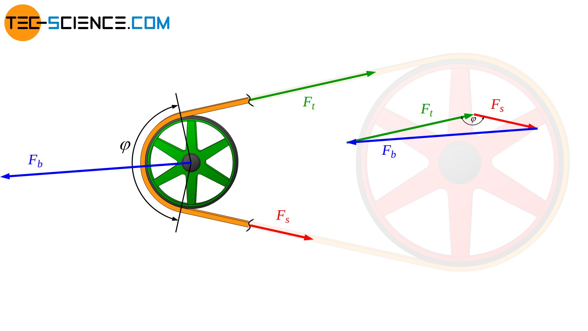
The forces acting in the belt press the belt onto the pulley and thus also act on the shaft bearings. The tight side force and the slack side force is thus balanced by the bearing force of the shaft. By the law of cosines, this bearing force Fb can be determined from the tight side force Ft and the slack side force Fs as well as from the wrap angle φ:
\begin{align}
\label{lagerkraft}
F_b=\sqrt{F_t^2 + F_s^2 – 2 \cdot F_t \cdot F_s \cdot \cos(\varphi)} \\[5px]
\end{align}
As shown in the article Calculation of the belt length, the wrap angle can be calculated using the diameter of the small and the large pulley (ds and dl) and the center distance e:
\begin{align}
\label{phi}
&\boxed{\varphi = \pi – 2 \cdot \arcsin\left( \frac{d_l-d_s}{2e}\right)} ~~~\text{ radian measure!} \\[5px]
\end{align}
If the tight side force and slack side force is expressed by the preload force Fp and the circumferential force Fc to be transmitted (see article Power transmission of a belt drive),
\begin{align}
\label{trumkraefte}
&F_t = F_p + \tfrac{F_c}{2} ~~~~~\text{and}~~~~~ F_s =F_p – \tfrac{F_c}{2} ~\text{,} \\[5px]
\end{align}
then the shaft load Fb can also be expressed as follows:
\begin{align}
&F_b=\sqrt{\left(F_p + \tfrac{F_c}{2} \right)^2 + \left( F_p – \tfrac{F_c}{2} \right)^2 – 2 \cdot \left(F_p + \tfrac{F_c}{2} \right) \cdot \left( F_p – \tfrac{F_c}{2} \right) \cdot \cos(\varphi)} \\[5px]
\label{F_W}
&\boxed{F_b=\sqrt{2 F_p^2 \cdot \left[1-\cos(\varphi) \right] + \tfrac{1}{2} F_c^2 \cdot \left[1+\cos(\varphi)\right] } } \\[5px]
\end{align}
In case the wrap angle is 180° (φ=π), the shaft load will be maximum, as the belt forces are then parallel and thus maximum effective. With cos(π)=-1 it follows directly from the equation above that the bearing load in later load operation corresponds to twice the value of the dynamic preload Fp:
\begin{align}
\label{wellenbelastung}
&F_{b,max}=2 \cdot F_p \\[5px]
\end{align}
The maximum bearing force corresponds to twice the value of the dynamic preload!
Influence of centrifugal forces on the bearing force
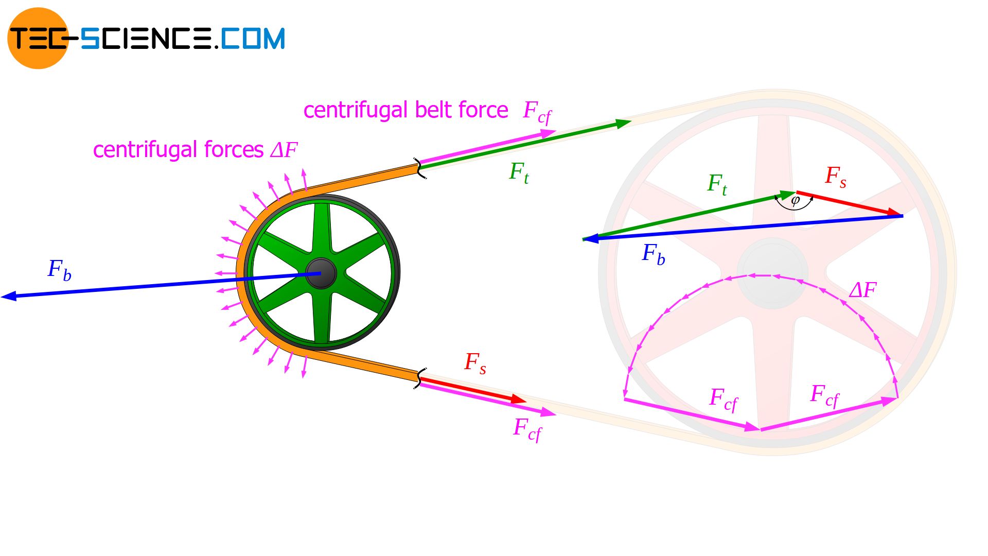
No centrifugal forces have to be taken into account for the calculation of the bearing force during operating! Although the belt must be tensioned more in advance by the amount of the expected centrifugal force, the additional centrifugal belt force does not affect the bearings in later operation, since the belt is attempted to lift off from the pulley with exactly this amount of force and thus relieves the bearing again to the same extent. The centrifugal forces acting on the belt and the additional centrifugal belt force acting in the belt form a closed polygon of forces and therefor cancel each other out. Only the dynamic preload Fp is relevant for the bearing force during operation.
The centrifugal forces existing during operation are compensated by the additional preload (centrifugal belt force) and therefore do not influence the bearing force!
Relationship between maximum circumferential force and bearing force
In the article Power transmission of a belt drive it could be shown that the maximum transmittable circumferential force Fc,max is related to the dynamic preload Fp by the following equation:
\begin{align}
\label{vorspannung}
&F_{p,min} = F_{c} \cdot \frac{e^{\mu \cdot \varphi}+1}{2 \left(e^{\mu \cdot \varphi} -1 \right) } ~~~ \text{or} ~~~\underline{F_{p} = F_{c,max} \cdot \frac{e^{\mu \cdot \varphi}+1}{2 \left(e^{\mu \cdot \varphi} -1 \right) }} \\[5px]
\end{align}
If equation (\ref{vorspannung}) is applied to equation (\ref{wellenbelastung}), the following relationship results between the existing bearing force Fb and the associated maximum transmissible circumferential force Fc,max:
\begin{align}
&F_b=2 \cdot F_{c,max} \cdot \frac{e^{\mu \cdot \varphi}+1}{2 \left(e^{\mu \cdot \varphi} -1 \right) } \\[5px]
&F_b=F_{c,max} \cdot \frac{e^{\mu \cdot \varphi}+1}{e^{\mu \cdot \varphi} -1} \\[5px]
\label{durchzugsgrad}
&F_{c,max} = F_b \cdot \frac{e^{\mu \cdot \varphi}-1}{e^{\mu \cdot \varphi} +1} \\[5px]
&\boxed{F_{c,max} = F_b \cdot \phi } ~~~~~\text{where}~~~~~\boxed{\color{red}{\phi = \frac{e^{\mu \cdot \varphi}-1}{e^{\mu \cdot \varphi} +1}}} ~~~\text{as “pull facor”} \\[5px]
\end{align}
The term marked in red in the equation above is also referred to as “pull factor” ϕ. For example, a pull factor 0.8 means that a maximum of 80 % of the bearing force acting in operation is available for the power transmission (strictly speaking only applies to parallel belt spans).
The higher the “pull factor”, the higher the maximum circumferential force compared to the bearing force, i.e. a high “efficient power transmission”!
Adjusting the preload by the bearing force
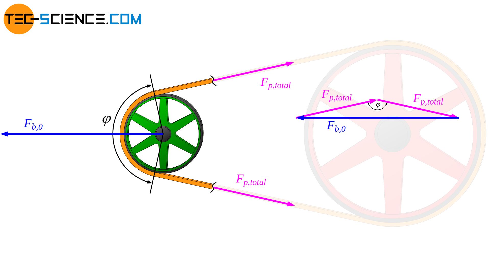
The pretension of the belt can be applied by adjusting the bearing force in the load-free state. In a load-free standstill, i.e. when no circumferential force is transmitted (Fc=0), the bearing load is determined only by the total preload force Fp,total (Note that in this case the total preload force also includes the centrifugal forces to be compensated!):
\begin{align}
&\boxed{F_{b,0}=F_{p,total} \cdot \sqrt{2 \left[1-\cos(\varphi) \right] } } \\[5px]
\end{align}
Thus, the total preload force Fp,total can be adjusted by the bearing force Fb,0 in the load-free state (or the preload force can be measured by the bearing force):
\begin{align}
&\boxed{F_{p,total}=F_{b,0} \cdot \frac{1}{\sqrt{2 \left[1-\cos(\varphi) \right] }} } \\[5px]
\end{align}


