Dissipative thermodynamic processes in adiabatic systems

In this article, learn more about dissipative thermodynamic processes using the polytropic equations.

Work performed in adiabatic systems

Many thermodynamic processes take place within very short times, such as the expansion of the burned fuel-air mixture in internal combustion engines during the power stroke (approx. 10 ms) or the expansion of hot gases in turbines. Within such short times, a significant heat transfer between gas and surroundings can be neglected in a first approximation (Q=0). The thermodynamic processes are then considered to take place in an adiabatic system. According to the first law of thermodynamics, the work done W by/on the gas is given directly by the change in internal energy ΔU of the gas:

\begin{align}
&\boxed{W+Q=\Delta U} &&~\text{first law of thermodynamics} \\[5px]
&W = \Delta U &&~\text{only applies to adiabatic systems (}Q=0 \text{)}\\[5px]
\end{align}

Since for ideal gases the change in internal energy ΔU is independent of the thermodynamic process and only results from the temperature change, …

\begin{align}
&\Delta U = c_\text{v} \cdot m \cdot \Delta T ~~~~~\text{where}~~~~~\Delta T = T_2-T_1\\[5px]
\end{align}

… the work done by/on the adiabatic system can be determined as follows:

\begin{align}
\label{9067}
&\boxed{W = c_\text{v}~m~\Delta T} ~~~\text{only applies to adiabatic systems (}Q=0 \text{)} \\[5px]
\end{align}

Note that the work denoted by W does not necessarily correspond to the pressure-volume work W_v of the gas. This would only be the case for a non-dissipative process where no friction occurs. Therefore, the work denoted by W describes quite generally the work transferred across the system boundary (boundary work) and thus also includes dissipative processes! More information about this can be found in the article Dissipation of energy in closed systems.

Equation (\ref{9067}) clearly shows that during the expansion of a gas in an adiabatic system, the greater the difference between the initial and final temperature, the more work is transferred from the system to the surroundings. For example, during the power stroke inside a diesel engine, the temperature in the cylinder drops from about 2000 °C to about 500 °C during expansion. However, at a given initial temperature T₁, dissipative processes with friction always lead to higher final temperatures T₂ compared to frictionless processes due to dissipation of energy that benefits the internal energy. The temperature obviously does not decrease as much during the expansion. Therefore, according to equation (\ref{9067}), the work done by the system ist lower!

Dissipative processes in the volume-pressure diagram

The volume-pressure diagram below shows an expansion of a gas in a cylinder which has been closed with a frictionless moving piston (blue curve). In comparison, an expansion is shown in which a constant frictional force between cylinder and piston was assumed over the duration of the expansion (red curve). It was assumed that the entire friction energy was dissipated in internal energy.

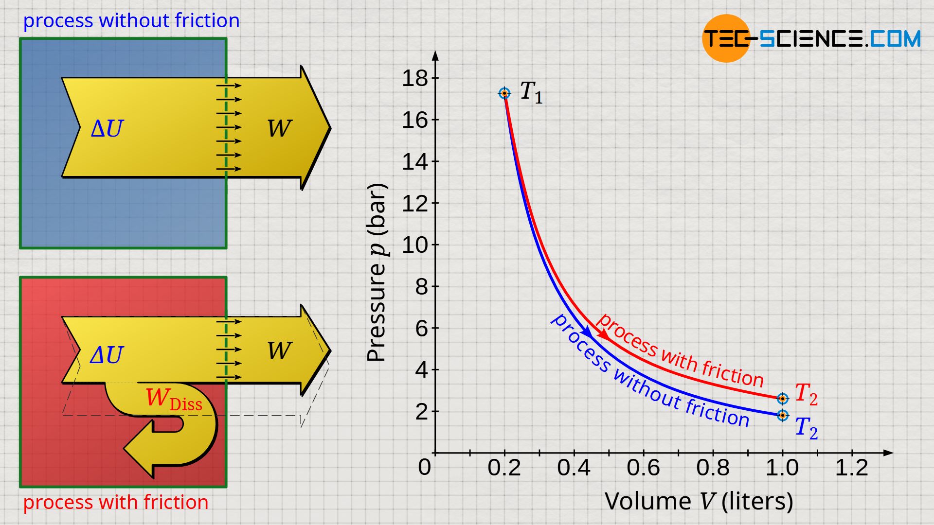
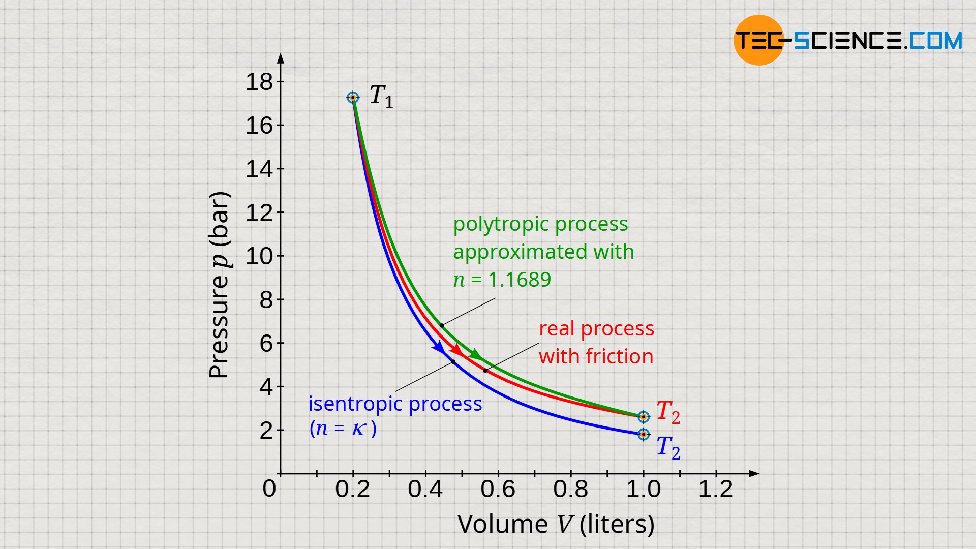
Due to the larger temperature difference, the greatest possible work is done by the gas during non-dissipative expansion → see equation (\ref{9067}). For such reversible processes, the laws of the isentropic process (n=κ) apply in adiabatic systems. Dissipative processes, on the other hand, run at a higher pressure level due to the higher temperatures. Such processes can then be approximated by a polytropic process, where in the case of an expansion the polytropic index n has a lower value than the isentropic index κ (n<κ):

\begin{align}
\label{3475}
&\boxed{p_1~V_1^n=p_2~V_2^n} \\[5px]
\label{2070}
&\boxed{T_1~V_1^{n-1}=T_2~V_2^{n-1}} \\[5px]
\label{9579}
&\boxed{T_1^n~p_1^{1-n}=T_2^n~p_2^{1-n}} \\[5px]
\text{ where: }~~ &n=\kappa ~~~\text{for non-dissipative (isentropic) processes} \nonumber \\
&n < \kappa ~~~\text{for dissipative (polytropic) expansion processes} \nonumber \\
&n > \kappa ~~~\text{for dissipative (polytropic) compression processes} \nonumber \\
\end{align}

With the use of these polytropic equations, the work W done by the system at a given initial temperature T₁ can also be determined by the pressure or volume ratio:

\begin{align}
\label{1}
&W=c_\text{v}~m~\left[T_2-T_1 \right] = c_\text{v}~m~T_1~\left[{T_2 \over T_1}-1 \right] \\[5px]
&\boxed{W=c_\text{v}~m~T_1~\left[{\left(V_1 \over V_2 \right)^{n-1}}-1 \right]}~~~\text{only applies to adiabatic systems} \\[5px]
\label{3}
&\boxed{W=c_\text{v}~m~T_1~\left[{\left(p_1 \over p_2 \right)^{{1-n} \over n}}-1 \right]}~~~\text{only applies to adiabatic systems} \\[5px]
\text{ where: }~~ &n=\kappa ~~~\text{for non-dissipative (isentropic) processes} \nonumber \\
&n < \kappa ~~~\text{for dissipative (polytropic) processes} \nonumber \\
\end{align}

At this point, it should be explicitly mentioned that one should refrain from using the term “adiabatic” process. This is because both the isentropic process (n=κ) and the polytropic process (n<κ) take place in an adiabatic system. In this respect, all these processes are “adiabatic”, but they differ, of course, due to the different polytropic index n used to describe the respective processes (see also the article Free expansion of an ideal gas in a vacuum)!

Calculation of the polytropic index for dissipative processes

Which polytropic index n best describes a given dissipative process can be determined on the basis of the initial and final states. In practice, of course, this requires an experimental determination of the respective values. Then either equation (\ref{3475}), equation (\ref{2070}), or equation (\ref{9579}) must be solved for the polytropic index n:

\begin{align}
\label{6526}
\boxed{n
=\frac{\ln{\left(\frac{p_2}{p_1}\right)}} {\ln{\left(\frac{V_1}{V_2}\right)}}
={\frac{\ln{\left(\frac{T_2}{T_1}\right)}} {\ln{\left(\frac{V_1}{V_2}\right)}} +1}
=\frac{\ln{\left(\frac{p_2}{p_1}\right)}} {\ln{\left(\frac{T_1}{T_2}\right)} + \ln{\left(\frac{p_2}{p_1}\right)} }
} \\[5px]
\end{align}

Based on the given initial and final state, a polytropic index of n=1.1689 seems to best reflect the dissipative process shown in the diagram (green curve). The comparison in the diagram below between the approximated polytropic process and the actual process (red curve) shows very good agreement at the beginning and towards the end of the process; however, there are minor deviations in the area in between.

Calculation of dissipated energy

In the article Dissipation of energy in closed systems it has already been explained in detail that the work W transferred across the system boundary (boundary work) is the sum of the pressure-volume work W_v of the gas and the dissipated energy W_diss due to friction:

\begin{align}
\label{ums}
&\boxed{W = W_\text{v} + W_\text{diss}} ~~~\text{work transferred across the system boundary}
\end{align}

In the article Polytropic process in a closed system, it was shown that the pressure-volume work W_v for a polytropic process can be determined using the following formula:

\begin{align}
\label{wv}
&\boxed{W_\text{v} = \left[{{\kappa-1} \over {n-1}}\right] ~c_\text{v}~m~\left(T_2-T_1 \right)}
\end{align}

Solving equation (\ref{ums}) for the dissipated W_diss energy and putting in equation (\ref{9067}) and equation (\ref{wv}), gives the dissipated energy:

\begin{alignat}{2}
\label{3440}
&W_\text{diss}= W – W_\text{v} = \underbrace{c_\text{v}~m~(T_2-T_1)}_{W} – \underbrace{\left[\frac{\kappa-1}{n-1}\right]~c_\text{v}~m~(T_2-T_1)}_{W_\text{v}} \\[5px]
\label{5715}
&\boxed{W_\text{diss}= \left[\frac{n-\kappa}{n-1}\right]~c_\text{v}~m~(T_2-T_1)} = \left[\frac{n-\kappa}{n-1}\right]~c_\text{v}~m~T_1~\left[{T_2 \over T_1}-1 \right] \\[5px]
\label{4461}
&\boxed{W_\text{diss}=\left[\frac{n-\kappa}{n-1}\right]~c_\text{v}~m~T_1~\left[{\left(V_1 \over V_2 \right)^{n-1}}-1 \right]} \\[5px]
\label{2394}
&\boxed{W_\text{diss}=\left[\frac{n-\kappa}{n-1}\right]~c_\text{v}~m~T_1~\left[{\left(p_1 \over p_2 \right)^{{1-n} \over n}}-1 \right]} \\[5px]
\end{alignat}

A closer look at these equations shows that they are the same equations that describe the transferred heat in a (non-dissipative) polytropic process (see article Polytropic process in a closed system). However, for the dissipative process at hand, they can no longer be interpreted as transferred heat, since the process takes place in an adiabatic system. However, the identical equations can still be explained from logic, because from an energetic point of view the dissipated energy has the same effect as a heat transfer, namely an increase of the internal energy!

Note

Note that the work W done by/on a closed system according to equations (\ref{1}) to (\ref{3}) depends only on the initial and final state. These equations therefore reflect the actual boundary work, even if the polytropic equations do not accurately describe the actual process (see diagram below). This is due to the fact that the initial and final values agree with reality, provided that the polytropic index was selected according to equation (\ref{6526})!

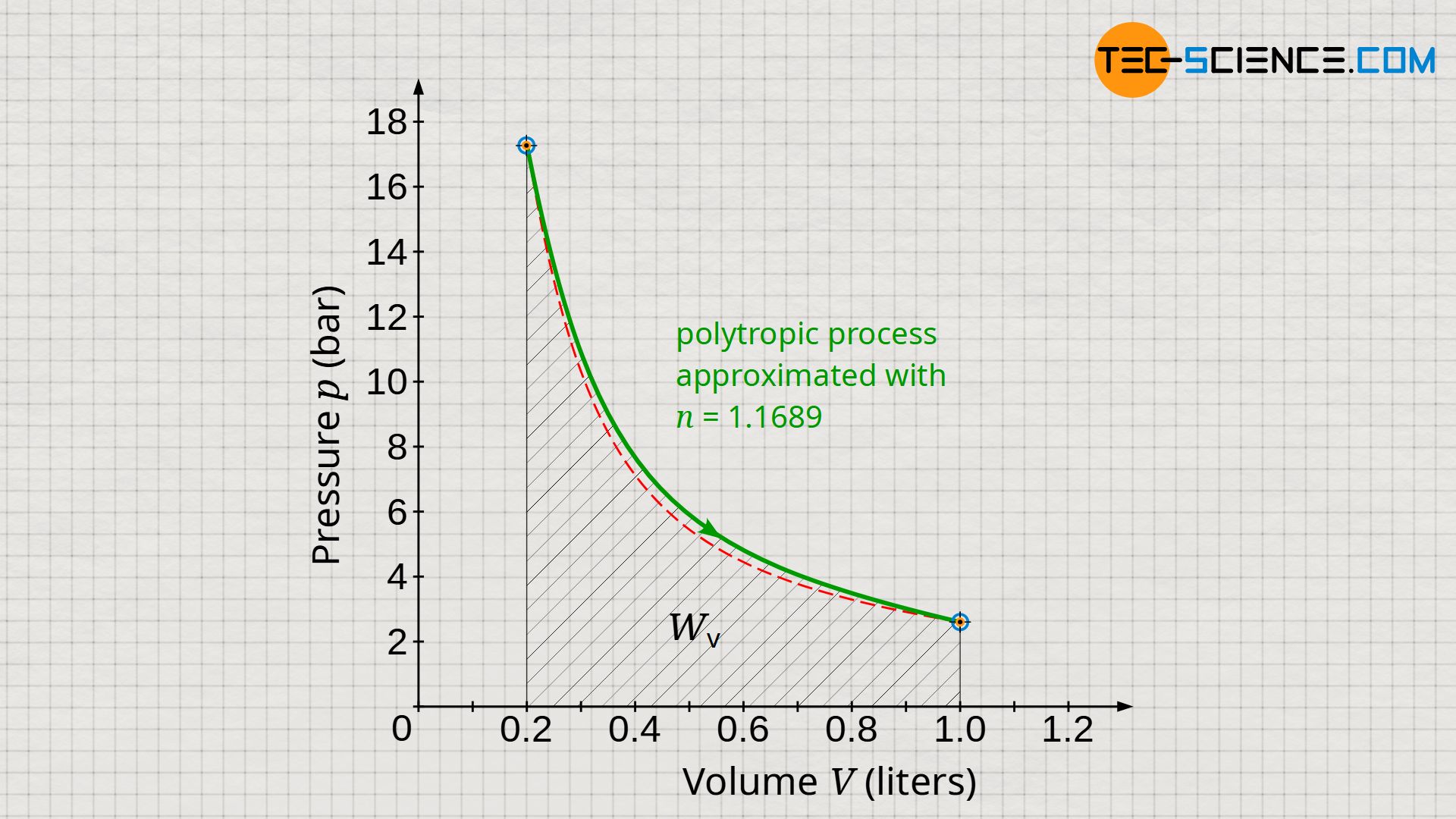
However, the situation is different for the dissipated work W_diss. For its determination, according to equation (\ref{3440}), the pressure-volume work W_v is relevant, which results as the area under curve in the volume-pressure diagram. However, as can be seen in the diagram, there are deviations between the approximated polytropic process and the actual process. Therefore, equations (\ref{5715}) to (\ref{2394}) will generally not accurately account for the dissipated energy. In the present case, the area under the polytropic curve is larger than for the actual process and thus suggests a somewhat larger dissipated energy than will be the case in reality.