In a bending flexural test, a standardized specimen is bent under uniaxial bending stress until plastic deformation or fracture occurs!
Test setup
In the bending flexural test, a specimen is loaded under uniaxial bending stress (tension and compression) in order to obtain information on the bending behaviour of materials. Especially brittle materials such as hard metals, tool steels and grey cast iron are tested in flexural tests. In such a bending test flexural strength, deflection at fracture and modulus of elasticity, for example, are determined.
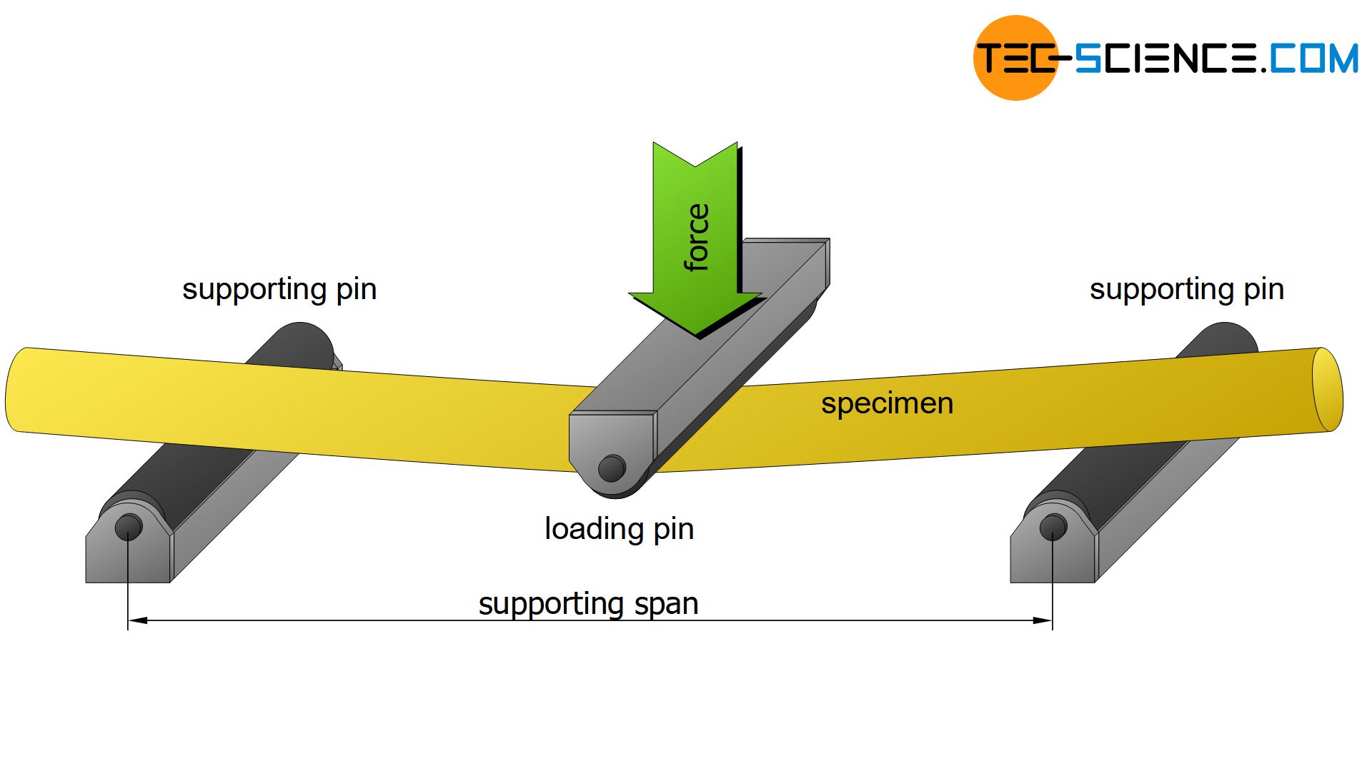
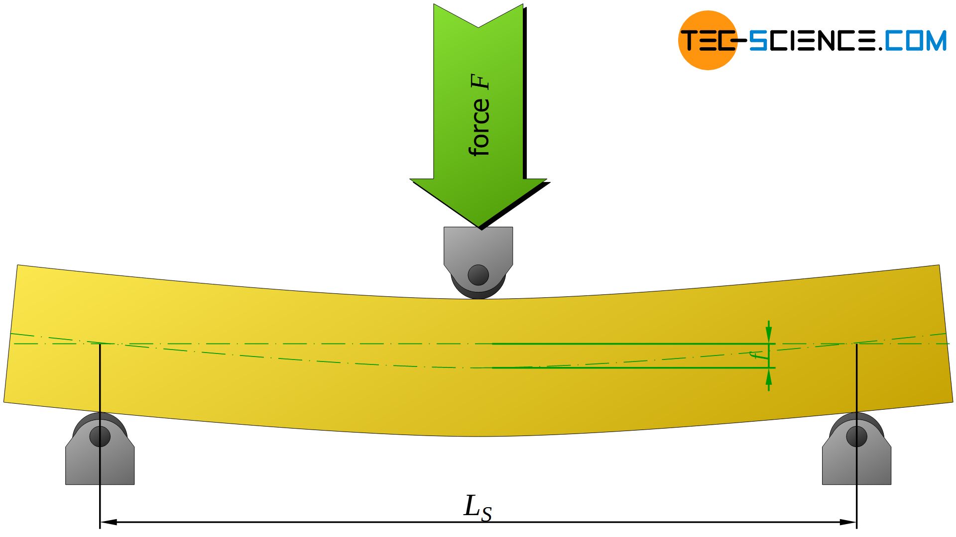
For this purpose, a standardized specimen is mounted on two supporting pins of a universal testing machine. A centrally arranged loading pin bends the specimen as the load increases. In general, round specimens with a circular cross-section are used whose diameters are in a certain ratio to the span between the pins (e.g. factor 20 for grey cast iron). Due to the three pressure points at the pins, this test arrangement is also called three-point flexural test.
In a flexural test, a standardized specimen is bent under uniaxial bending stress until plastic deformation or fracture occurs in order to obtain information about the flexural behaviour of materials!
Stress distribution
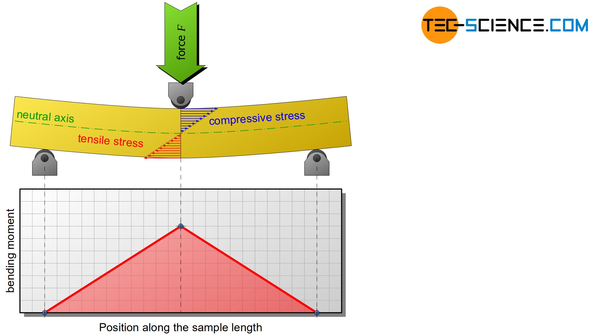
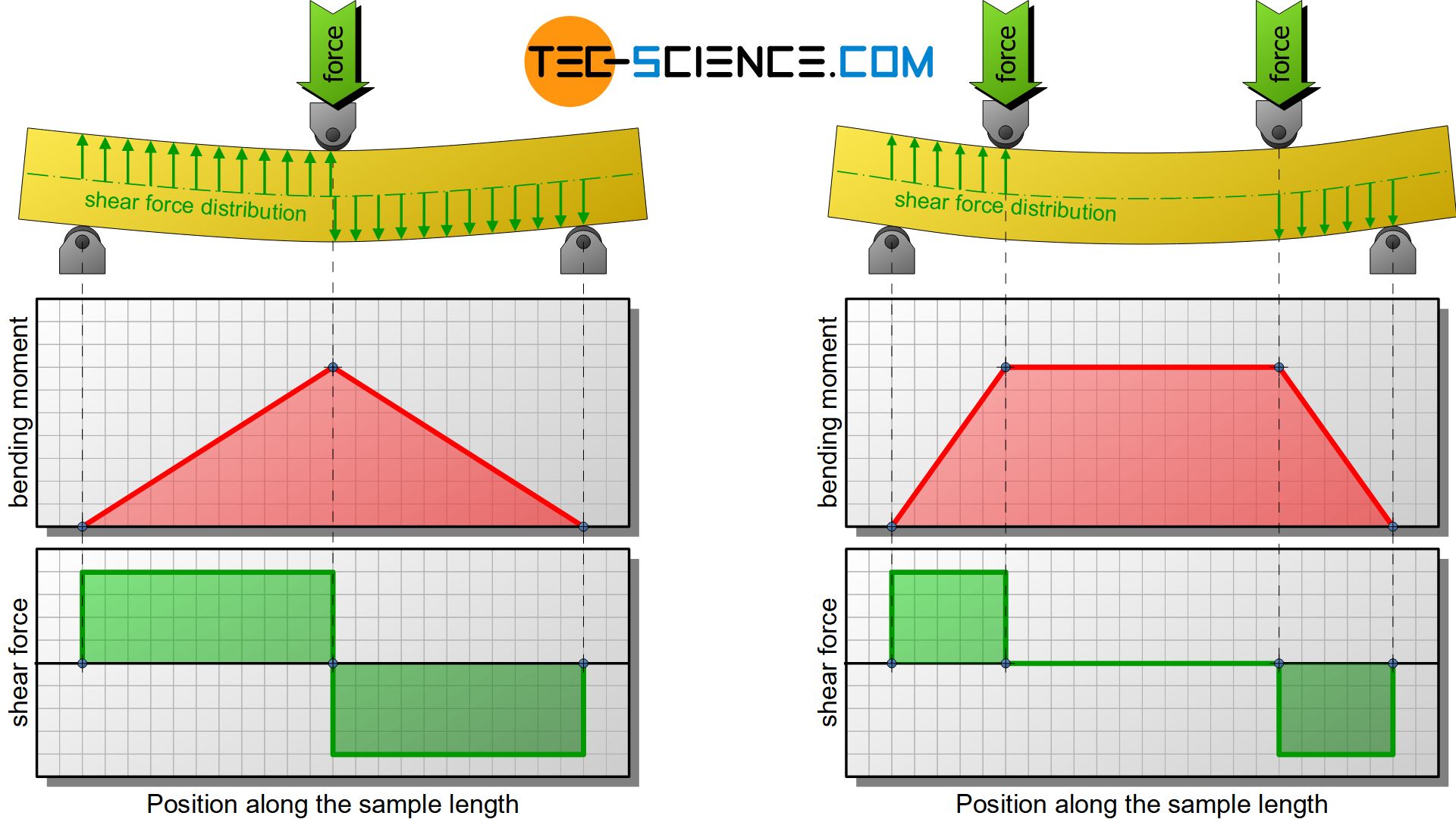
The bending load has its highest value in the cross section of the maximum deflection, i.e. in the middle of the specimen. The highest torque (moment) is located there. In the present case of bending this moment is also called bending moment. Starting from the center of the specimen, the bending moment decreases linearly up to the two supporting pins. The diagram below shows the corresponding course of the bending moment and the shear force over the entire specimen length.
The maximum bending moment \(M_b\) at the point of maximum deflection is determined by the force \(F\) acting there and the span \(L_S\) as follows:
\begin{align}
\label{biegemoment}
&\boxed{M_{b} = \frac{F \cdot L_S}{4}} ~~~~~[M_b]=\text{Nmm} \\[5px]
\end{align}
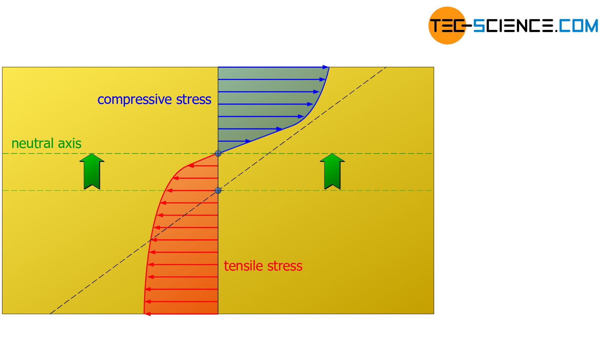
While the material is stretched on the outside of the curvature, compression takes place on the inside. As a result, the material is subjected to compressive stress on the inside and tensile stress on the outside. The stress values are highest at the surface layer of the material due to the maximum compression or strain. The stresses decrease inwards in each case. Within the elastic limit and especially when Hooke’s law is obeyed, this results in a linear stress dependency.
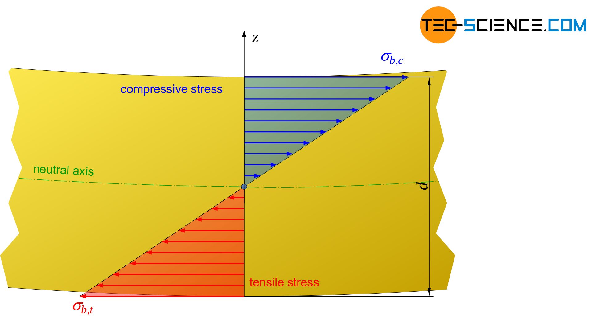
The material remains unstressed at the transition from tensile to compressive stress. This characterizes the so-called neutral axis. In materials that react equally to a tensile and a compressive stress, the neutral axis passes through the geometric center of gravity of the specimen cross-section. In this case, the tensile and compressive stresses are distributed identically over the cross-section.
The material is not subjected to tensile or compressive stress in the neutral axis and therefore remains unstressed there!
The decisive factor for failure under bending stress are always the stresses occurring in the surface layers, since the highest stress values are located there. These maximum stresses are sometimes just referred to bending stresses \(\sigma_b\). Compared to the tensile or compression test, in which the stresses are distributed homogeneously over the specimen cross-section, the flexural test shows an inhomogeneous stress distribution, which is influenced equally by tensile and compressive forces. It can therefore be assumed that different strength values apply to a material under bending stress than in the tensile or compression test.
The tensile and compressive stresses increase linearly starting from the neutral axis up to the surface of the material and become maximum there. These maximum stresses are decisive for the loading of the material and are called bending stresses!
In order to be able to define limit values for the bending stresses, these must first be described mathematically using the external load (bending moment). This will be discussed in more detail in the next section.
Bending stresses
In the previous section, the the linear stress distribution caused by a bending load was explained. This section focuses on its mathematical description, in particular the determination of the maximum stresses \(\sigma_b\) (bending stresses) at a given bending moment \(M_b\).
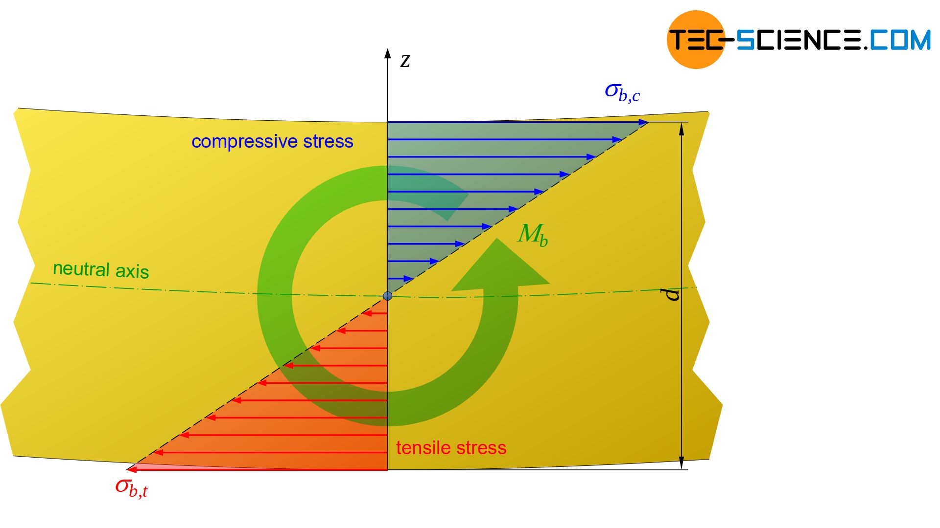
In principle, the total tensile and compressive stresses inside the material cause an internal moment which is balanced with the external bending moment \(M_b\). From this equilibrium analysis, a relationship between the bending moment \(M_b\) and the resulting stress \(\sigma\) at a distance \(z\) from the neutral axis can be established, depending on the specimen cross-sectional geometry (a linear stress distribution is assumed!). The cross-sectional geometry is characterized by the so-called area moment of inertia \(I\) (also referred to as second moment of area).
\begin{align}
\label{biegegleichung}
&\boxed{\sigma = \frac{M_b}{I} \cdot z} ~~~~~[\sigma]=\frac{\text{N}}{\text{mm²}} ~~~~~\text{only valid in the linear-elastic range} \\[5px]
\end{align}
The area moment of inertia for a circular cross-section is determined solely by its diameter \(d\):
\begin{align}
\label{flaechentraegheitsmoment}
&\underline{I = \frac{\pi \cdot d^4}{64}} ~~~~~[I]=\text{mm}^4 ~~~~~\text{area moment of inertia for circular cross-sections} \\[5px]
\end{align}
Note: Equation (\ref{biegegleichung}) is only valid if the strain in the elastic range is proportional to the induced stresses and thus results in a linear stress distribution in the cross-section (linear-elastic range). In particular, this means that the law of Hooke is obeyed. Whether this assumption is always justified will be discussed later.
The bending stresses \(\sigma_b\) occurring at the surface can now be determined with the bending equation (\ref{biegegleichung}) with \(\tfrac{d}{2}\) for the distance \(z\). The quotient of second moment of area \(I\) and distance \(\tfrac{d}{2}\) (which are solely geometry parameters) is referred to the so-called section modulus \(W_a\), which consequently also represents solely a geometric characteristic value.
\begin{align}
&\underline{\sigma_b} = \frac{M_b}{I}\cdot \frac{d}{2} = \frac{M_b}{\tfrac{2\cdot I}{d}} = \underline{\frac{M_b}{W_a}} ~~~~~ \text{with} ~~~~~ \underline{W_a = \frac{2\cdot I}{d}} \\[5px]
\end{align}
For a circular cross-section with the diameter \(d\), the section modulus \(W_a\) is calculated as follows:
\begin{align}
\label{axiales_widerstandsmoment}
&\underline{W_a = \frac{\pi \cdot d^3}{32}} ~~~~~[W_a]=\text{mm}^3 \\[5px]
\end{align}
For non-circular cross-sections, the respective second moment of areas or section moduli can be looked up in table books. Thus, the bending stress \(\sigma_b\) resulting from a given bending moment \(M_b\) can now be determined with the following formula using the section modulus of the specimen:
\begin{align}
\label{biegespannung}
&\boxed{\sigma_b = \frac{M_b}{W_a}} ~~~~~[\sigma]=\frac{\text{N}}{\text{mm²}}\\[5px]
\end{align}
Note that this bending equation is only valid within the linear-elastic range!
The mathematical relationship between the applied bending moment and the bending stresses induced in the surface region is determined by the section modulus which is purely dependent on the cross-section geometry!
With this mathematical determination of the bending stresses, strength limits can now be determined in the flexural test which must not be exceeded.
Testing of ductile materials
As long as the bending stress is below the limit of the plastic deformation, the specimen is subjected to purely elastic stress. As the load increases steadily, the critical stress is first exceeded in the marginal areas (exceeding the “yield point”). Then, there will be a plastic deformation in the surface layers. This plastic deformation is also called flowing.
The regions further inside the material are theoretically exposed to a purely elastic deformation with regard to the effective stress. However, this has no practical significance, because if the deformation in the edge area is maintained even after the force has been removed, the supposedly “elastic” deformed regions are ultimately remain as well. Residual stresses are formed in the specimen (more on this see section stress distribution within the plastic range).
The limit to which ductile materials can be stressed at a given bending load without permanent deformations in the edge area is called flexural yield strength \(\sigma_{by}\). This yield point for bending is determined by the (\ref{biegespannung}) with the applied bending moment \(M_{by}\) at the onset of plastic deformation and the section modulus \(W_a\) of the specimen cross-section:
\begin{align}
\label{biegefliessgrenze}
&\boxed{\sigma_{by} = \frac{M_{by}}{W_a} } ~~~~~\text{flexural yield strength} \\[5px]
\end{align}
Flexural yield strength is the limit bending stress from which plastic deformation begins in the margin area!
To determine the onset of plastic deformation, the deflection is measured as a function of the applied force and recorded in a deflection-force diagram. Force and deflection are determined directly at the loading pin or rather via its travel.
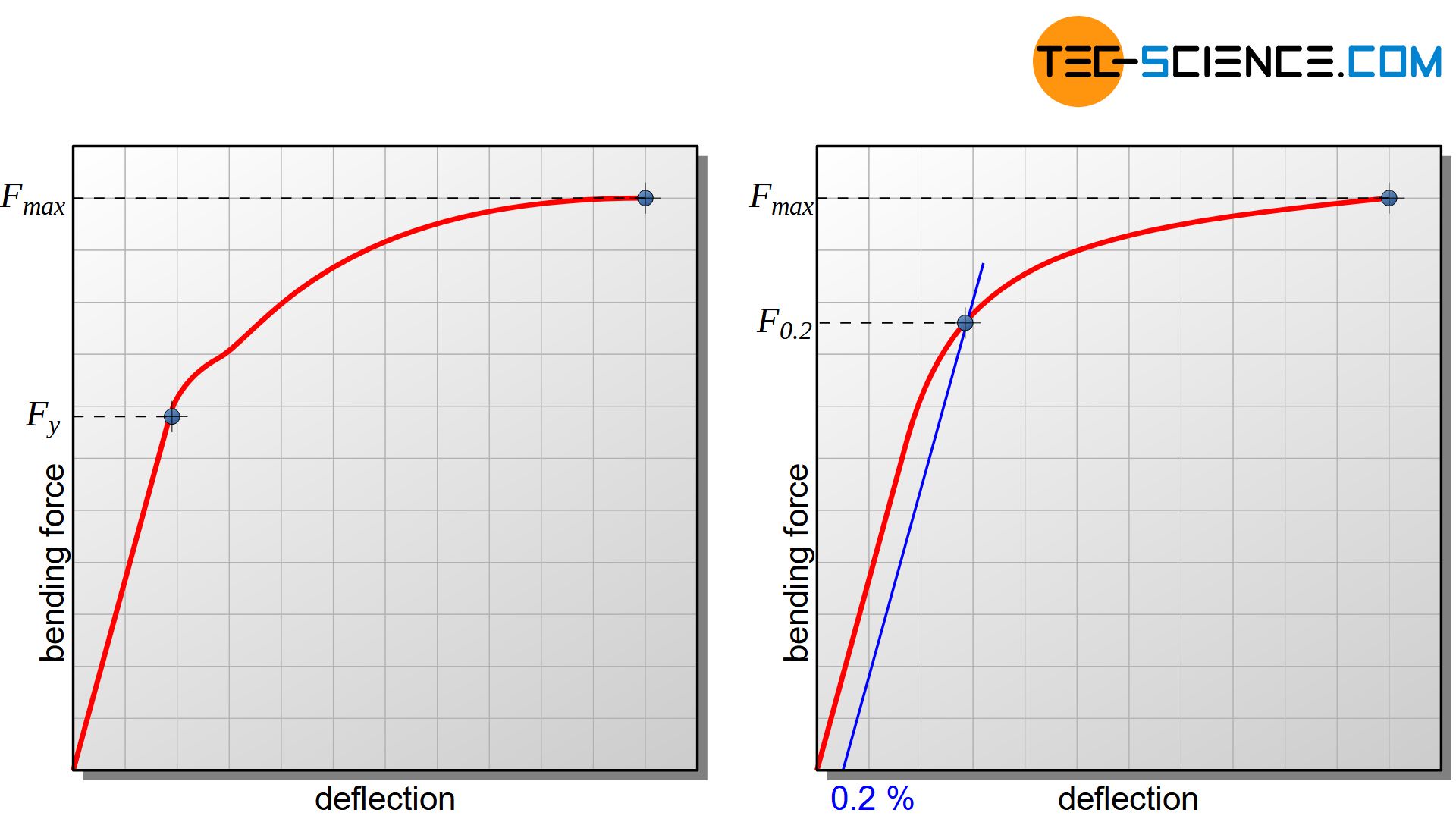
At the beginning of the measurement, there is a proportional relationship between the applied force and the resulting deflection. Only elastic deformations occur in this linear range. When the elastic limit is exceeded, the curve flattens out as in the stress-strain diagram of the tensile test and indicates the yield force \(F_y\). With this yield force the induced bending moment \(M_{by}=\tfrac{F_y \cdot L_S}{4}\) can be determined at the onset of plastic deformation and thus the flexural yield point according to the equation (\ref{biegefliessgrenze}).
However, a pronounced yield point as in the tensile test (short-term decrease in force after the start of plastic deformation) is usually not obtained in the force-deflection-diagram of the flexural test. Due to the characteristic stress curve in the specimen cross-section, the areas further inside are are not at once but increasingly involved in the deformation process with a constantly increasing deflection. It is therefore not a one-off start of the plastic deformation process over the entire cross-section but a gradual involvement.
This also results in the flexural yield strength usually being about 10 % to 20 % higher than the (tensile) yield strength. Thus, when the tensile yield point is exceeded in the marginal areas, the areas that are still subjected to purely elastic stress further inside cause an obstruction of the plastic deformation. They exert a kind of supporting effect and thus ensure that the yield point is shifted to slightly higher values. The flow process therefore only starts at higher marginal stresses than the tensile test with its yield point suggests!
Due to the linear stress distribution at a bending load, the flexural yield strength for steels is about 10 % to 20 % higher than the tensile yield strength!
For materials with no visible yield strengths in the stress-curves, a 0.2 % flexural offset yield strength \(\sigma_{by0.2}\) can be defined analog to the 0.2% offset yield strength of the tensile test. This yield point is determined by the bending equation (\ref{biegegleichung}), although, the linear stress distribution is no longer valid and therefore this equation as well. Thus, the flexural offset yield point is ultimately a fictitious stress value and does not correspond to the true stress value (more on this see section stress distribution within the plastic range):
\begin{align}
\label{biegedehngrenze}
&\boxed{\sigma_{by0.2} = \frac{M_{by0.2}}{W_a} } ~~~~~\text{flexural offset yield strength} \\[5px]
\end{align}
In this equation \(M_{by0.2}\) corresponds to the bending moment at which a permanent deformation of 0.2 % occurs at the most stressed point.
With tough materials, the specimen can continue to be plastically deformed as the load increases, but cannot be fractured. The deformability is so pronounced that the specimen would only be pulled through the two supporting pins. For tough materials, the flexural test is therefore terminated when the flexural yield point is exceeded.
Testing of brittle materials
Compared to ductile materials, brittle samples usually show a different behavior in flexural tests. The sample often breaks without any noticeable deformation. Determining a flexural (offset) yield point is difficult for such materials. Therefore, in the case of brittle materials, it is not the onset of plastic deformation that is used as the material strength but the onset of fracture when the maximum bending moment \(M_{b,max}\) is reached. This strength parameter is then called (ultimate) flexural strength or bending strength or modulus of rupture \(\sigma_{bu}\).
Bending strength or flexural strength is the maximum bearable bending stress at which the specimen fractures!
The bending strength is also determined according to the bending equation (\ref{biegegleichung}), although in the state of fracture there is no longer a linear stress distribution due to plastic deformation! In particular, the law of Hooke’s is no longer obeyed and the cross-sections no longer remain even. The flexural strength is therefore a purely fictitious value which does not correspond to the true bending stress in the material (more on this see section stress distribution within the plastic range)!
\begin{align}
\label{biegefestigkeit}
&\boxed{\sigma_{bu} = \frac{M_{b,max}}{W_b} } ~~~~~[\sigma_{bB}]=\frac{\text{N}}{\text{mm²}} ~~~~~\text{flexural strength} \\[5px]
\end{align}
In addition to the bending strength, the so-called fracture deflection \(f_b\) can be determined for brittle materials, which indicates the maximum deflection of the specimen immediately before fracture. This value must of course always be considered in relation to the span \(L_S\), since larger spans in principle mean larger deflections.
A valid statement about the strength of brittle materials can usually be better made on the basis of the flexural test than on the tensile test. The reason for this is the pronounced bending sensitivity when the specimen is clamped at an angle in the tensile test. In contrast to tough materials, a misalignment of brittle materials can (almost) not be compensated by deformation. Even when the specimen is slightly tilted, very high bending stresses occur, which cause the specimen to break prematurely due to the combined stress of tension and bending.
For the determination of the strength of brittle materials, the flexural test is usually more suitable than the tensile test!
The flexural test can therefore be more suitable than the tensile test for testing the strength of brittle materials, since the material is exposed to a pure bending load. However, this statement must be somewhat relativized, because although the 3-point bending test is the most common, it has the disadvantage that in addition to the induced tensile and compressive forces, lateral forces (shear stresses) also act in the material.
For this reason, the four-point flexural test was developed. The single loading pin is just substituted by a double pin. Between these points there is a shear force-free range with a constant bending moment.
Determination of the Young’s modulus
In addition to the strength parameters such as flexural yield point or flexural strength, the flexural test can also be used to determine the modulus of elasticity (Young’s modulus). The dependence of the specimen deflection on the Young’s modulus of the material is used, provided that the deflection is of a purely elastic nature. Without going to deeply into the bending theory of beams and their underlying assumptions, the elastic deflection \(f_{el}\) of the specimen center is given by the following equation for slim specimens in the 3-point bending test:
\begin{align}
\label{durchbiegung}
&\boxed{f_{el} = \frac{F_{el} \cdot L_S^3 }{48 \cdot E \cdot I} } ~~~~~[f]=\text{mm} \\[5px]
\end{align}
Note that this equation is only valid within the elastic range!
In this equation \(F_{el}\) denotes the applied test force (in N), \(L_{S}\) the span (in mm), \(E\) the modulus of elasticity (in N/mm²) and \(I\) the area moment of inertia of the specimen cross-section (in mm4). Looking at the equation (\ref{durchbiegung}) it becomes apparent that the greater the product of Young’s modulus \(E\) (material property) and area moment of inertia \(I\) (geometric property), the less the specimen deflects. For this reason, this product is often referred to as bending stiffness \(B\) (flexural rigidity). The bending stiffness is neither a pure material parameter nor a pure geometric parameter, but ultimately a “specimen parameter”.
\begin{align}
\label{biegesteifigkeit}
&\boxed{B = E \cdot I} ~~~~~[B]=\text{N mm²} ~~~~~\text{bending stiffness} \\[5px]
\end{align}
If the equation (\ref{durchbiegung}) is solved for the modulus of elasticity, the Youngs modulus \(E\) can be determined as follows from the applied test force \(F_{el}\) and the resulting deflection \(f_{el}\):
\begin{align}
\label{emodul}
&\boxed{E = \frac{F_{el} \cdot L_S^3 }{48 \cdot f_{el} \cdot I} } ~~~~~[E]=\frac{\text{N}}{\text{mm²}} ~~~~~\text{Youngs modulus} \\[5px]
\end{align}
Stress distribution within the plastic range
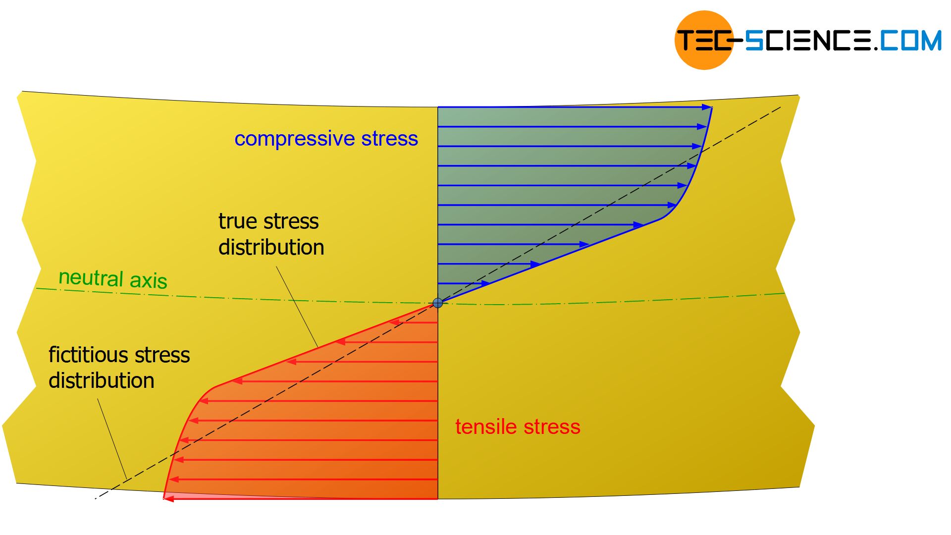
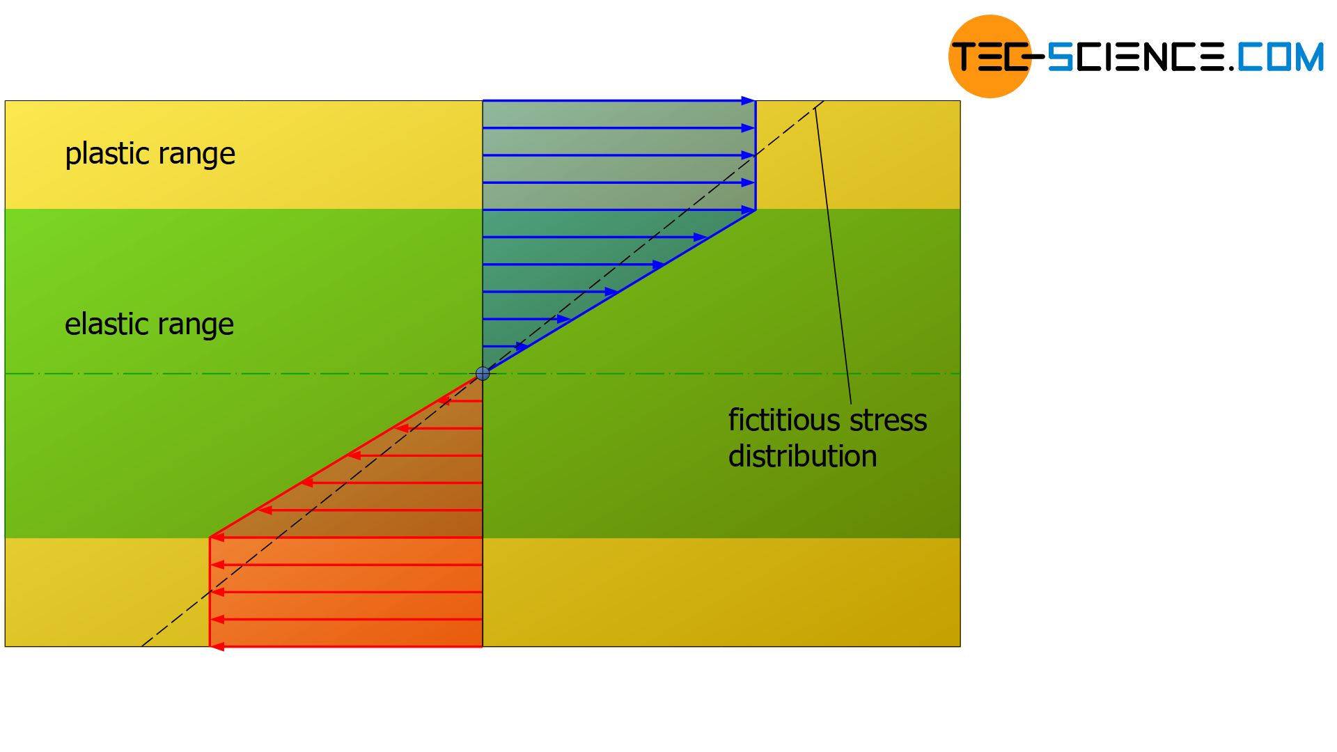
As already explained in detail, the stress distribution in the cross-section of a specimen subjected to purely elastic bending stresses has a linear course, provided that Hooke’s law applies to the materials. However, this changes when the elastic limit (flexural yield strength) is exceeded. For materials without strain hardening effects, the stress in the outer areas does not increase further when the yield point is exceeded. If the bending moment is increased again, the areas further inside are only stressed up to the maximum flexural yield point.
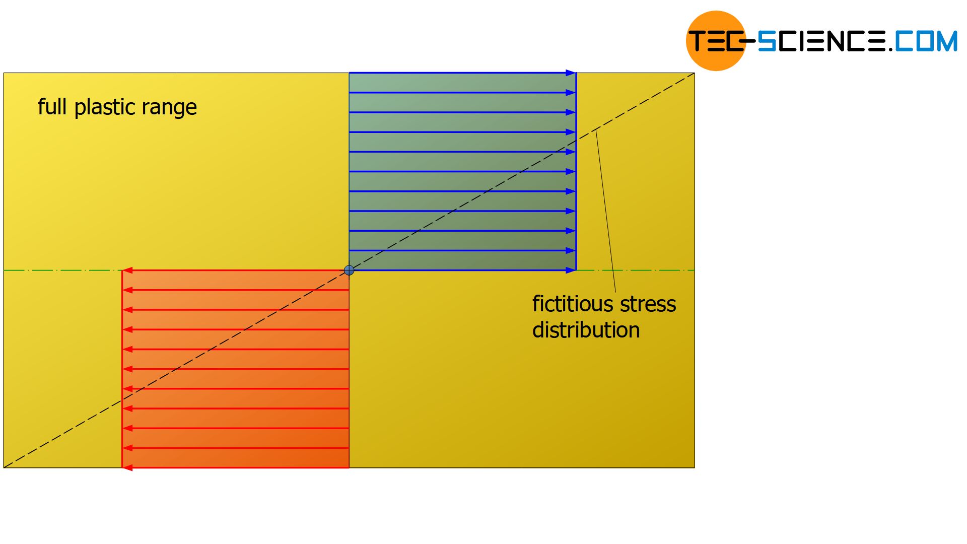
The following figures show the fictitious stress distribution with a dashed line that generates the same internal moment (necessary for the equilibrium) as the actual stress distribution.
In the case of materials which show strain hardening during plastic deformation, the stress increases when the yield point is exceeded in accordance with the hardening effect. As a result of the increase in hardening, the stress curve gradually flattens out from the point at which the yield strength is exceeded. On the other hand, the stress increases more strongly in the elastic range, but retains the typical linear stress distribution near the neutral axis. In the extreme case of a fully plastic state, i.e. when theoretically the entire cross-section is deformed to a maximum extent, the stress distribution changes into a rectangular shape.
During plastic deformation, the stress is no longer distributed linearly over the cross-section. Equation (\ref{biegespannung}), which was derived assuming the linear stress distribution, can therefore no longer be used to determine the bending stress in the surface layers!
If this equation is nevertheless used to determine the stress values, the calculated (fictitious) stresses in the outer regions are greater than the actual stresses (see dashed line in the figures). Inside the sample, however, the calculated stresses are smaller than those actually effective. In particular, this means that the bending strengths determined by means of equation (\ref{biegespannung}) are basically greater than the bending stresses actually present at fracture.
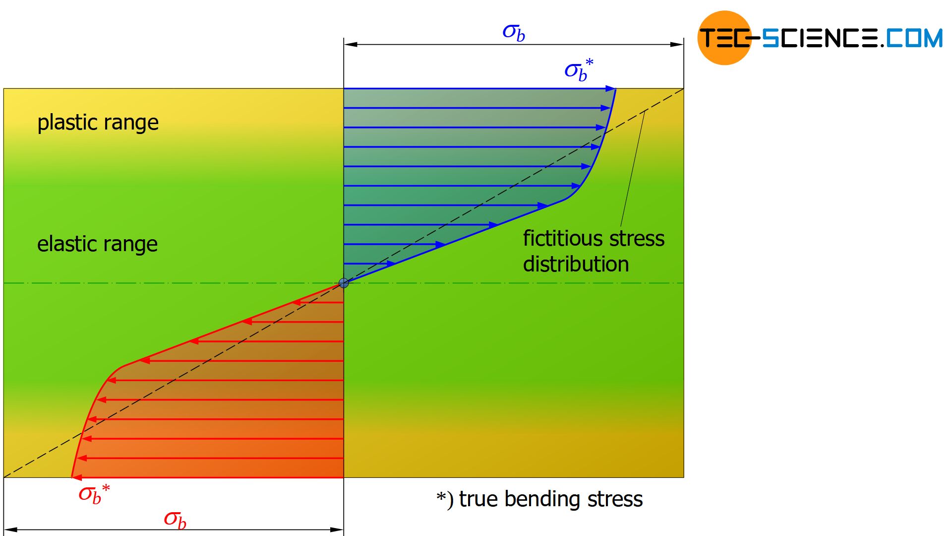
In the case of plastic deformation the bending stresses calculated with the bending equation (e.g. in the case of bending strength) are greater than the actual stresses present!
Residual stresses induced by plastic deformation
If a partially plastically deformed specimen is relieved in the flexural test, only the internal stresses or only the internal torque act at this moment. This results in a re-forming of the sample. The internal stresses try to restore the elastically deformed areas of the sample to their original state, while the plastically deformed areas prevent exactly this. Even without external forces, stresses remain in the material, which are then referred to as residual stresses.
When relieving a plastically deformed specimen, residual stresses remain in the material!
Since the fictitious stress curve is based on the validity of Hooke’s law with its elastic deformation behaviour, the residual stresses can be determined from the difference between the true stress and the fictitious stress (“reshaping of the elastic components”). New neutral axis are formed which are neither subjected to tensile nor compressive stress.
Stress distribution for grey cast iron
The stress distribution under bending load for grey cast iron shows a specialty. This material shows a dependence of the Young’s modulus on the stress. Hooke’s law is longer obeyed! Grey cast iron also reacts differently to a tensile load than to a compressive load. Grey cast iron can withstand compressive stresses to a much greater extent than tensile stresses. Accordingly, there will also be a different stress distribution which, overall, has higher compressive stress values than tensile stress values.
Nevertheless, for static reasons, the compressive force resulting from the distribution of compressive stress must be equal in amount to the tensile force resulting from the distribution of tensile stress. However, since the tensile stresses are at an overall lower level, they must therefore cover a larger cross-sectional area in order to meet the static equilibrium. The unequal stress distribution therefore causes the neutral axis to shift from the geometric center of gravity of the cross-sectional area towards the area of compression.
In the case of grey cast iron, the neutral axis shifts towards the area of compression!


")
")
")